
Strictly feasible sum-of-squares solutions
A question on the YALMIP forum on the SeDuMi homepage essentially boiled down to how can I generate sum-of-squares solutions which really are feasible, i.e. true certificates?
This is partially answered and discussed in one of the sum-of-squares examples and the referenced paper Löfberg 2009. The problem boils down to the fact that semidefinite solvers typically work with infeasible methods. Hence, the optimal solution you obtain in the end is very often slightly infeasible.
The semidefinite programs
When YALMIP sets up a sum-of-squares problem, there are two alternative approaches. The first approach, which is used by default, is the kernel representation, sometimes called primal form in YALMIP. You can explicitly tell YALMIP to use this form by setting sos.model to 1 in sdpsettings when calling solvesos.
An alternative approach, which typically is the approach seen when using pen and paper, is the image representation, also called dual form. This form is typically less efficient computationally, but is easier to understand, and is the only applicable method when parametric variables have advanced constraints, such as integer constraints or additional nonconvex constraints. YALMIP use this form by setting the option sos.model to 2. Of course, the data (C,A,b,F,f) is different in the two models, otherwise it would make no difference since most solvers solve the primal and the dual problem simultaneously.
The default value of the sos.model option is 0, which means that YALMIP makes the decision (almost always primal form).
As mentioned earlier, most SDP solvers work with infeasible methods. In practice, this means the equality constraints in the primal form typically are violated in the final solution, and the semidefinite constraint in the dual form is not satisfied. If the optimization problem originates from a sum-of-squares problem, this means the SDP solution has failed to create a true certificate of positivity, all it has done is shown that it is very close to being a sum-of-squares.
In the dual form, the sum-of-squares certificate is theoretically useless when the semidefinite constraint is violated. In primal form, it can be shown that it is possible to prove sum-of-squareness holds despite violation of constraints, by relating the smallest eigenvalue of \(X\) to the largest violation of the equality constraints, see [Löfberg 2009].
Hence, we would like to force the SDP solver to return a feasible solution, or even better, a significantly strictly feasible solution (assuming you have created a model for which such a solution really exists).
An example
As an example, consider the problem of finding a lower bound on \(p(x,y) = (1+xy)^2-xy+(1-y)^2\) over the box \(-5\leq (x,y)\leq 5 \) and \(-5 \leq y\leq 5 \)
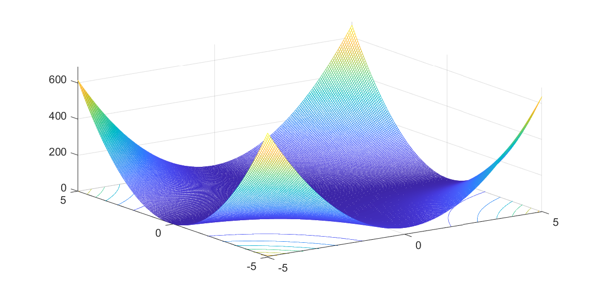
Define the polynomial \(p(x,y)\) and the constraints \(g(x,y)\geq 0\) defining the box
sdpvar x y
p = (1+x*y)^2-x*y+(1-y)^2;
g = [5-x;5+x;5-y;5+y]
To solve the problem, we will apply the postivstellensatz using quadratic multipliers. Hence, we define 4 parameterized multiplier polynomials
[s1,c1] = polynomial([x y],2);
[s2,c2] = polynomial([x y],2);
[s3,c3] = polynomial([x y],2);
[s4,c4] = polynomial([x y],2);
We apply standard sum-of-squares arguments and solve the following problem, for simplicity using the image representation.
sdpvar lower
Constraints = [sos(p-lower-[s1 s2 s3 s4]*g), sos(s1), sos(s2), sos(s3),
sos(s4)];
Params = [c1;c2;c3;c4;lower];
ops = sdpsettings('sos.model',2);
[sol,v,Q] = solvesos(Constraints,-lower,ops,Params);
For this to really be a certificate, all Gramians, returned in the output ‘'’Q’’’, should be positive semidefinite. This is however not the case for most solvers.
>> min(eig(Q{1}))

ans =

   -9.634448808807465e-009
Close to 0 and the optimal value of the lower bound is probably correct (within reasonable tolerances), but we really do not have a true certificate.
To overcome this, one trick is to use the fact that semidefinite solvers typically return solutions in the analytic center of the feasible region, when a feasibility problem is solved, i.e., if a strict interior exists, we will obtain a strictly feasible solution. A feasibility problem will however not return an optimal solution, of course. To circumvent this, we add a new constraint forcing the solver to return a feasible solution which is very close to optimal value. Hence, we resolve the problem with the requirement that we should be within 1/10000 from the previously computed optimal objective value.
FeasibilityConstraints = [Constraints, lower >= 0.99999*value(lower)];
[sol,v,Q] = solvesos(FeasibilityConstraints,[],ops,Params);
Indeed, a strictly feasible (very close to optimal) solution is returned
>> min([eig(Q{1});eig(Q{2});eig(Q{3});eig(Q{4});eig(Q{5})])
ans =
   1.2738e-007
For the default case when the kernel model is used, the fourth argument from solvesos, the residuals from the equality constraints, have to be involved in the analysis, see [Löfberg 2009].
Note that this whole discussion here only is relevant if you absolutely have to have a true numerical certificate. In most cases, if the solver finishes without any complaints and the solution is slightly infeasible, it is up to your discretion to judge if it can be used anyway.