interp1

interp1 overloads interp1, with additional flags for a creating mixed-integer sos2-based approximation or standard convex epigraph representations.

Syntax

y = interp1(xdata,ydata,x,'method')

Example (Nonlinear optimization)

Create a nonlinear function over a grid and find the global minima of a spline interpolated version of the nonlinear function, using the global solver BMIBNB.

xi = (-5:.1:5);
yi = sin(xi) + cos(xi.^2).*sin(xi).^2

sdpvar x
y = interp1(xi,yi,x,'spline');
optimize([],y,sdpsettings('solver','bmibnb'));
plot(xi,yi);hold on;
xii = (-5:0.001:5);
plot(xii,interp1(xi,yi,xii,'spline'));
plot(xii,sin(xii) + cos(xii.^2).*sin(xii).^2)
plot(value(x),value(y),'k*')

Alternatively, we can use a linear interpolation (still implemented as a nonlinear function using a callback framework)

y = interp1(xi,yi,x,'linear');
optimize([],y,sdpsettings('solver','bmibnb'));
plot(xi,yi);hold on;
xii = (-5:0.001:5);
plot(xii,interp1(xi,yi,xii,'linear'));
plot(xii,sin(xii) + cos(xii.^2).*sin(xii).^2)
plot(value(x),value(y),'k*')

In this particular case could have worked with the nonlinear function directly which most likely is more efficient as it is composed of very simple operators.

y = sin(x)+cos(x^2)*sin(x)^2
optimize([-5 <= x <= 5],y,sdpsettings('solver','bmibnb'))
plot(value(x),value(y),'r*')

And of course, gridding univriate function followed by optimization over an interpolant makes absolutely non sense, as we just could have used the data to begin with

[y_min,loc] = min(yi);
xi(loc)

Example (Linear optimization)

With the flags ‘sos2’ or ‘milp’ a sos2 representation of the piecewise affine function interpolating the supplied data points is created, and thus requires a sos2-capable mixed-integer linear solver.

y = interp1(xi,yi,x,'milp');
optimize([],y)

For problems where the data represents a convex (or concave) function and convexity of the problem can be derived, we can (and should!) use a simple linear epigraph (hypograph) representation. This is obtained with the flag ‘graph’. YALMIP will automatically analyze the data and the problem to check convexity. Note that the approximator will create hyperplanes going through neighbouring data points, and thus create an upper approximation of convex functions, and a lower approximation of concave functions

yi = 15*xi.^2 - xi.^3 + 20*xi;
y = interp1(xi,yi,x,'graph');
optimize([],y);
clf;
plot(xii,interp1(xi,yi,xii,'linear'));
hold on
plot(value(x),value(y),'r*')

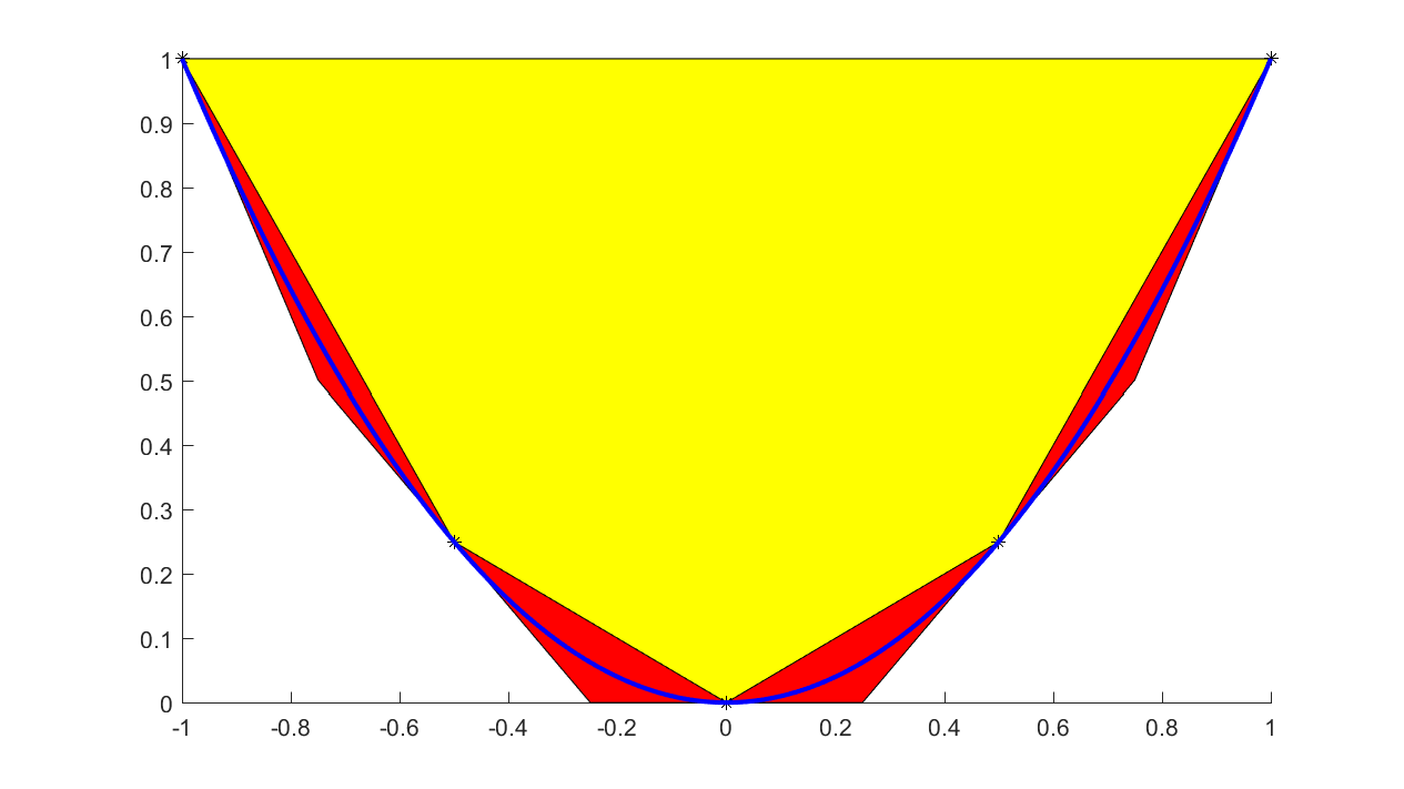
When talking about graph models, one typically thinks of tight underestimators for convex functions. Hence, a more natural piecewise affine approximation is based on tangent cuts, instead of interpolation. This can be achieved by supplying an additional input with derivatives. To see the difference between these models, we approximate a quadratic coarsely using both interpolants and tangents to generate the hyperplanes

xi = -1:1/2:1;
yi = xi.^2;
dyi = 2*xi;

sdpvar x f
f = interp1(xi,yi,x,'graph',dyi);
plot(f <= 1,[x;f]);hold on
f = interp1(xi,yi,x,'graph');
plot(f <= 1,[x;f],'yellow');

xifine = -1:0.001:1;
yifine = xifine.^2;
l = plot(xifine,yifine,'b')
plot(xi,yi,'k*')

If convexity assumptions fail, an error will be generated. If we want YALMIP to adaptively select between an efficient linear graph model and a MILP based model, we use the flag ‘lp’ instead.

yi = 15*xi.^2 - 2*xi.^3 + 20*xi;
y = interp1(xi,yi,x,'lp');
optimize([],y);
clf;
plot(xii,interp1(xi,yi,xii,'linear'));
hold on
plot(value(x),value(y),'r*')

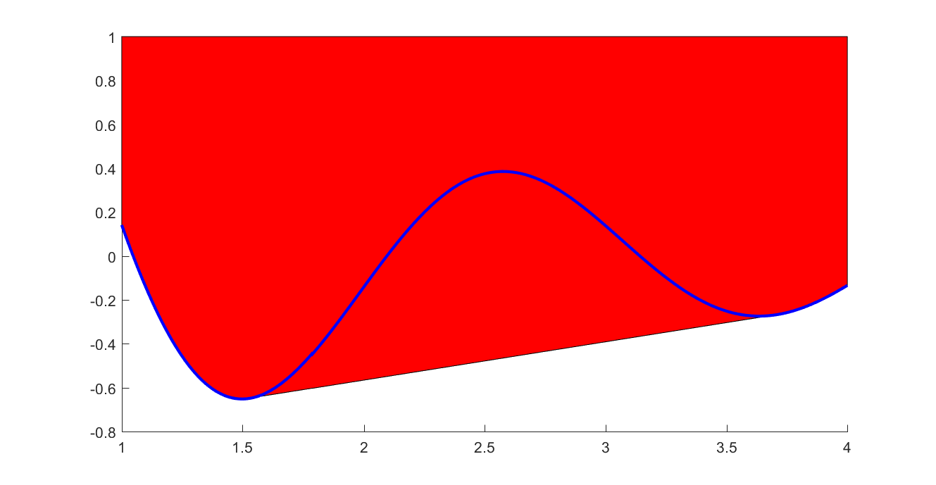
If you have nonconvex data, but want to create a linear epigraph representation of the lower convex envelope, you can use the flag ‘envelope’ and the data will automatically be pruned

xi = 1:0.01:4;
yi = sin(3*xi)./xi;

sdpvar x f
f = interp1(xi,yi,x,'envelope');
plot(f <= 1,[x;f]);hold on

xifine = 1:0.001:4;
yifine = sin(3*xifine)./xifine;
plot(xifine,yifine,'b')

Example (Nonlinear optimization)

The normal case is as above whre we have given data, and use that directly to define an approximating function. Another scenario could be that we have data we want to approximate, but we first want to select an optimal approximator by tuning the data used to define the approximation. This can be handled since the data defining the interpolating function can be decision variables.

Assume we have a function (q(x)) we want to approximate using a spline (f(x). To judge the approximation, we will use the performance measure ( \int_{-1/2}^1 (q(x)-f(x))^2 dx), and that integral will be approximated by a rectangle approximation evaluated on a fine grid.

q = @(x)x.^2+min(0,8*x);
x = -0.5:0.05:1;

We want to use a very simple spline interpolant defined from only 4 data points. To improve performance, we will not use the function values obtained by evaluating in the grid points, but we will let these be decision variables, and try to optimize them.

N = 4;
xi = linspace(-.5,1,N);
yi = sdpvar(1,N);
method = 'spline';
fi = interp1(xi,yi,x,method);

Define the approximation of the integral, and optimize!

objective = sum((q(x)-fi).^2);
optimize([],objective);

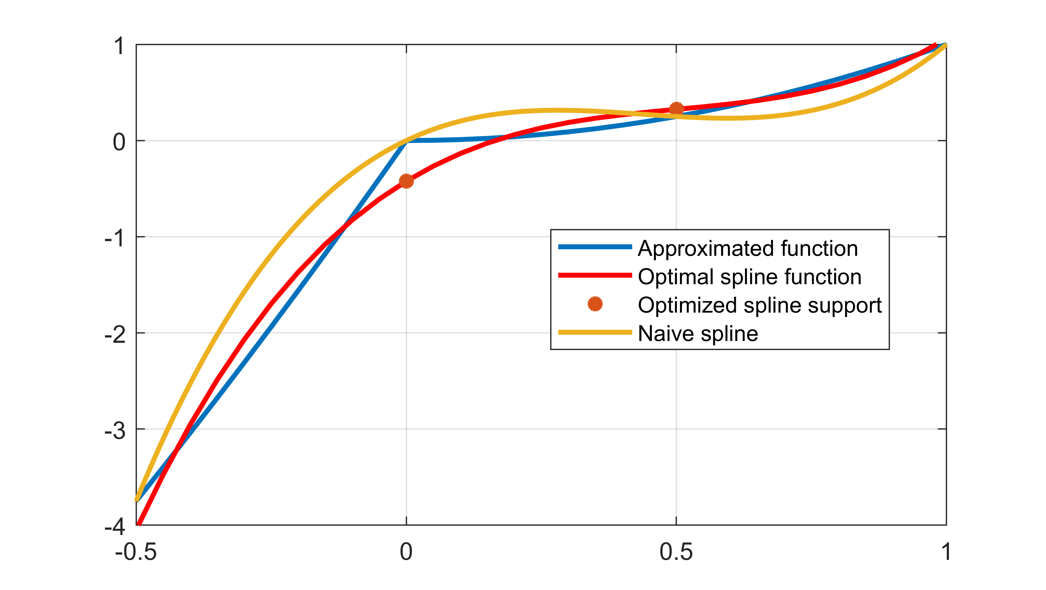
The computed spline is far better than a naive spline when using the integral squared error as a metric

plot(x,q(x));
plot(x,interp1(xi,value(yi),x,method))
plot(xi,value(yi),'*');
plot(x,interp1(xi,q(xi),x,method))
legend('Approximated function','Optimal spline function','Optimized spline support','Naive spline')

The standard spline will give a spline which goes through the supplied function values. We can make the comparison slightly more fair by constraining our spline to be consistent with data in the end-points

Model = [interp1(xi,yi,x(1),'spline') == q(x(1)),
         interp1(xi,yi,x(end),'spline') == q(x(end))]
optimize(Model,objective);
plot(x,q(x));
plot(x,interp1(xi,value(yi),x,method))
plot(xi,value(yi),'*');
plot(x,interp1(xi,q(xi),x,method))
legend('Approximated function','Optimal spline function','Optimized spline support','Naive spline')

Implementation

In the nonlinear case when the operator is implemented using the callback framework, the operator does not compute derivatives, which can lead to slow computations (and in general, computing a single function value is expensive).