The CUTSDP solver explained

YALMIP is shipped with two built-in mixed-integer conic programming solvers, both relying on external solvers to do the heavy work, but in completely different ways.

The most known solver is the solver BNB, which is a classical branch-and-bound implementation for mixed-integer convex programs (it can applied to any problem, but global optimality guarantees only hold for problems where the continuous relaxations are convex). The solvers are only relevant for mixed-integer semidefinite programs. For all other problem classes there are much better external solvers.

A less known internal mixed-integer solver is CUTSDP. While BNB is based on branch-and-bound where, roughly speaking, integrality is approximated and relaxed during the iterative process, CUTSDP is based on an iterative process where the geometry of the semidefinite cone is approximated and relaxed during the process, while integrality is guaranteed throughout.

Cutting planes - from the semidefinite cone to linear elementwise cone

CUTSDP is not only a solver for mixed-integer conic (second-order and semidefinite) programs, but is a general solver for conic programs also in the continuous case (although one should never use it as such).

The basic idea is simple, and is a classical approach to nonlinear programming. A semidefinite constraint \(X\succeq 0\) is by definition equivalent to the infinite-dimensional linear programming model \(v^TXv \geq 0 ~ \forall~v\). The trick now is to cleverly generate a lot of vectors \(v\) and construct a linear program, such that the geometry of the linear programming model starts to approximate the geometry of the semidefinite program. Every such added linear constraint is called a cutting plane. Note that the linear program is an outer approximation of the original semidefinite program. This means that a feasible solution to the linear programming approximation is not guaranteed to be a feasible solution to the semidefinite program. It also means that if we are minimizing an objective, it will generate a lower bound.

To see the basic idea in practice, we consider a simple semidefinite constraint defining a ball, and an objective which tells us we want to go as far as possible to the nort-east, and then approximate this model with an increasing number of cutting planes (to speed up the process, we add 20 cutting planes before plotting again. To see a faster high-level implementation, look at this post). Note also that almost all time here is spent on plotting the set.

sdpvar x y
% Manual SDP model of x^2 + y^2 <= 1
X = [1 x y;[x;y] eye(2)];
Objective = -x-y;
ops = sdpsettings('plot.shade',.1,'verbose',0);
% Initial outer approximation
ballApproximation = [-1 <= [x y] <= 1];
clf;hold on
for k = 1:10  
  for i = 1:20
    vi = randn(3,1);
    ballApproximation = [ballApproximation, vi'*X*vi >= 0];  
  end
  plot(ballApproximation,[x;y],'blue',200,ops); 
  optimize(ballApproximation,Objective,ops);
  plot(value(x),value(y),'k*');drawnow
  drawnow
end 

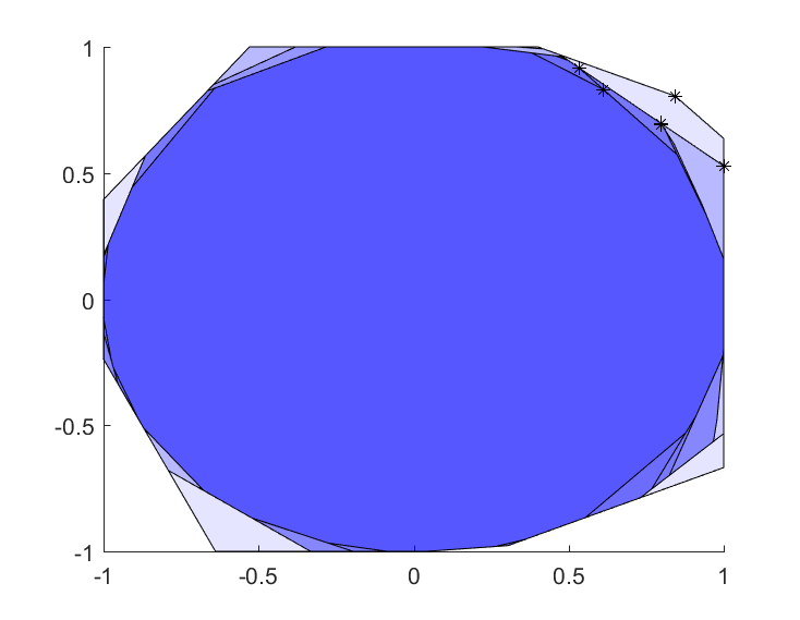
Creating a solver based on this strategy is primarily about generating relevant cutting planes, instead of randomly placing them everywhere. Since we have an objective function, we are not interested in approximating the whole feasible set, but only need a good approximation around the (unknown) optimal point. Additionally, as it is in the implementation above, we are generating new cuts which might be completely redundant, i.e., they do not cut away any infeasible points.

Consider a solution leading to a matrix \(X^{\star}\). If the solution is infeasible with regards to the semidefinite constraint, we know that the smallest eigenvalue of \(X^{\star}\) is negative. Hence there is a negative \(\lambda\) and a vector \(v\) such that \(X^{\star}v = \lambda v\),. i.e., \(v^TX^{\star}v = \lambda v^Tv < 0\). In other words, the current solution violates the constraint \(v^TXv \geq 0\). This indicates that eigenvectors \(v\) associated with negative eigenvalues for the current semidefinite constraints are suitable candidates for creating cutting planes.

ballApproximation = [-1 <= [x y] <= 1];
clf;hold on
for k = 1:10  
  optimize(ballApproximation,Objective,ops);
  [V,D] = eig(value(X));  
  vi = V(:,1);
  ballApproximation = [ballApproximation, vi'*X*vi >= 0];    
  plot(ballApproximation,[x;y],'blue',200,ops);   
  plot(value(x),value(y),'k*');
  drawnow
end 

In a very few steps, the semidefinite constraint is sufficiently well approximated around the true optimal solution, and the problem is solved. Of course, this particular problem is trivial, and for real problems the number of cutting planes can grow very large while still having large infeasibility (negative eigenvalues in the semidefinite constraints).

The CUTSDP solver implements precisely this strategy, generalized to multiple constraints, and second-order cone constraints.

Adding integrality constraints

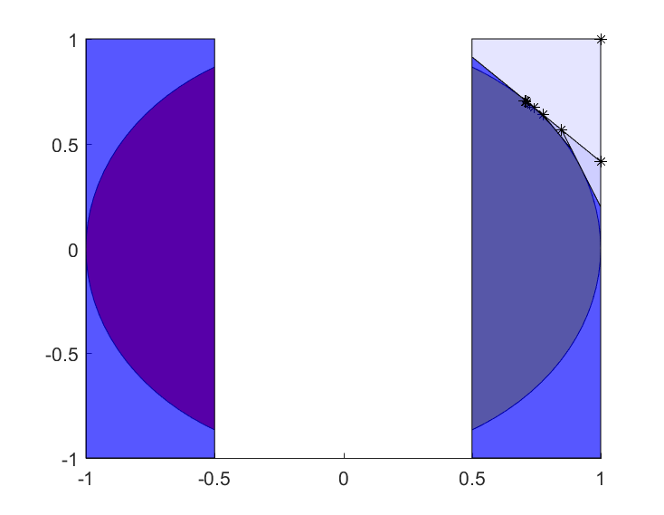
If we now add integrality constraints to the model, nothing really changes. We are still outer approximating the semidefinite cone, but instead of solving linear programs, we will solve mixed-integer linear programs. If the solution to the mixed-integer program satisfies the original semidefinite program, it is our sought solution. If not, it must violate some semidefinite constraint, and we can add a cutting plane based on a negative eigenvalue. Note that a purely integer semidefinite program is a mixed-integer linear program in disguise. The feasible set is the integer lattice points, and the convex hull of these is a polytope.

Let us create a mixed-integer semidefinite program, which models a problem where we are in one of two half-moons, which can be cast as a mixed-integer semidefinite program (in practice you would write it using a quadratic constraint and YALMIP would derive a mixed-integer second-order cone problem instead). You must have an efficient mixed-integer linear programming solver installed for the cutting-plane iterations to be fast, and you need a semidefinite-programming solver installed for the first plot to be generated. The integrality in the model comes from the use of combinatorial implications with the binary variable defining in which half-moon we are.

clf
hold on
X = [1 x y;[x;y] eye(2)];
binvar d
plot([X >= 0, -1 <= [x y] <= 1, implies(d,x>=0.5),implies(1-d,x <= -0.5)]);
Model = [-1 <= [x y] <= 1, implies(d,x>=0.5),implies(1-d,x <= -0.5)];
for i = 1:10
    plot(Model,[x;y],'yellow',200,ops)
    optimize(Model,-x-y,ops);
    plot(value(x),value(y),'k*');drawnow
    [V,D] = eig(value(X))
    v = V(:,1);
    Model = [Model, v'*X*v >= 0];
end

A direct implementation with CUTSDP to solve this problem would be

Model = [x^2 + y^2 <= 1,
        -1 <= [x y] <= 1, 
        implies(d,x>=0.5),implies(1-d,x <= -0.5)];
optimize(Model, Objective, sdpsettings('solver','cutsdp'));        

Should I use bnb or cutsdp

It really depends on the problem. BNB relaxes integrality but handles the semidefinite geometry exactly, while CUTSDP relaxes the semidefinite cone while it handles integrality exactly in every iteration. Depending on the geometry of your problem, they will behave differently. Always test both.