Big-M and convex hulls

YALMIP has some support for logic programming (implies, nnz, sort, alldifferent etc) and structured nonconvex programming (nonconvex use of operators such as min , max, norm, abs etc.) This feature relies on converting the user supplied model to an internal mixed-integer model, typically a mixed-integer linear program. The method used for performing this conversion is big-M reformulations.

In most of the examples related to logic programming and nonconvex models, the importance of explicit bounds is stressed, and this example will try to motivate why this is important, describe the basics of big-M reformulations, and show how you manually can create stronger models by using the hull command.

Big-M reformulations

Big-M reformulations are used to convert a logic or nonconvex constraint to a set of constraints describing the same feasible set, using auxillary binary variables and additional logic constraints.

As an example, consider the logic constraint if y == 1 then x==0 where y is binary and x is a continuous variable, which in YALMIP is written as implies(y,x==0). A big-M reformulation of this constraint would be

[(1-y)*m <= x <= (1-y)*M]

If M is chosen sufficiently large and m is sufficiently small (i.e., negative and large in absolute terms), this big-M reformulation is equivalent to the original constraint. If y is 1 (true), the only feasible x is 0, and our goal is accomplished. The complications arise when y is 0 and x should be unconstrained. For x to be unconstrained in this case, M has to be a number larger than any possible value that x can take in the complete model, and m smaller than any possible value of x. This is where the name big-M comes from.

Hence, for a big-M reformulation to work, the modeling language has to be able to derive these constants, or conservative approximations, from the complete model. YALMIP derives these constants from the model automatically by searching for simple variable bound constraints and using these bound constraints to compute conservative bounds on the expressions involved in the big-M constraint. Consequently, you have to add explicit bounds on all variables that are involved in logic constraints or constraints involving nonconvex instances of operators such as max, min etc.

Note: The term big-M is devastatingly misleading, and a better term would be sufficiently-large-small-M. A naive (and sadly commonly used) approach is to use huge constants without any thought, such as M=1e6 and m=-1e6. This works in theory, but will give extremely bad and essentially useless models. The big-M reformulations will result in terrible numerics in solvers, and the relaxations that are used in the mixed integer solver will be very weak, leading to excessive branching and thus increased computation time. As we will see in this example, already with modestly sub-optimal choices, the relaxations are terrible.

Nonconvex polytope constraints

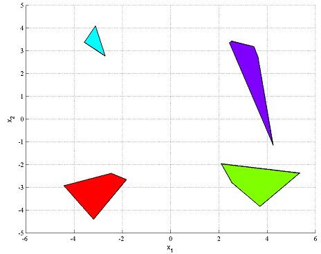
To illustrate the importance of tight bounds for the big-M reformulations, we will optimize over the union of polytopes.

Define numerical data for four random polytopes.

x = sdpvar(2,1);
n = 10;
A1 = randn(n,2);
b1 = rand(n,1)*2-A1*[3;3];
A2 = randn(n,2);
b2 = rand(n,1)*2-A2*[-3;3];
A3 = randn(n,2);
b3 = rand(n,1)*2-A3*[3;-3];
A4 = randn(n,2);
b4 = rand(n,1)*2-A4*[-3;-3];
plot(A1*x<=b1)
plot(A2*x<=b2)
plot(A3*x<=b3)
plot(A4*x<=b4)

Constraining a variable x to be in the union of the four polytopes, can be done easily in YALMIP by using the overloaded OR operator

F = [(A1*x <= b1) | (A2*x <= b2) | (A3*x <= b3) | (A4*x <= b4)];

When this is done, the nonlinear operator framework is used, and the model is converted to a big-M model when the problem is solved. We will however do the modelling by hand here, to illustrate the underlying problems.

The big-M model for this case is easy to derive, and is easily seen to be given by the following model.

x = sdpvar(2,1);
d = binvar(4,1);
M1 = 1000;
M2 = 1000;
M3 = 1000;
M4 = 1000;
F = [sum(d) == 1];
F = [F, A1*x - b1 <= M1*(1-d(1))];
F = [F, A2*x - b2 <= M2*(1-d(2))];
F = [F, A3*x - b3 <= M3*(1-d(3))];
F = [F, A4*x - b4 <= M4*(1-d(4))];

A problem with this model is that we have naively picked the big-M constants large (at least we think they are large enough), without insight to the problem. The consequence of this is (except the poor numerics) the weakness of the relaxed mixed integer model. We can see this by plotting the relaxed feasible set and compare it with the actual feasible set.

plot(F,x,[],[],sdpsettings('relax',1))
hold on
plot(A1*x<=b1)
plot(A2*x<=b2)
plot(A3*x<=b3)
plot(A4*x<=b4)

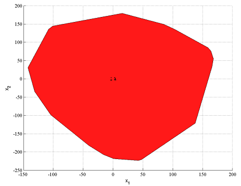
The relaxation is far from a good approximation of the true feasible set, indicating that a mixed integer solver may have problems solving this problem efficiently, since it typically relies on strong relaxations.

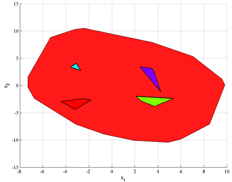
A better model is obtained by using a more reasonable big-M constant (In this example, it is hard to use a good constant since the data is randomly generated. In practice, realistic bounds which is needed for YALMIPs derivation typically follow from model insight (When YALMIP performs the modeling internally, a considerable amount of preprocessing is performed in order to derive good bounds, based on supplied bounds on the involved variables)

M1 = 50;
M2 = 50;
M3 = 50;
M4 = 50;
F = [sum(d) == 1];
F = [F, A1*x - b1 <= M1*(1-d(1))];
F = [F, A2*x - b2 <= M2*(1-d(2))];
F = [F, A3*x - b3 <= M3*(1-d(3))];
F = [F, A4*x - b4 <= M4*(1-d(4))];
clf
plot(F,x,[],[],sdpsettings('relax',1))
hold on
plot(A1*x<=b1)
plot(A2*x<=b2)
plot(A3*x<=b3)
plot(A4*x<=b4)

As stated above, in practice YALMIP takes care of the modelling. All the user has to do is to supply good variable bounds.

F = [(A1*x <= b1) | (A2*x <= b2) | (A3*x <= b3) | (A4*x <= b4)];
F = [F, -20 <= x <= 20];
clf
plot(F,x,[],[],sdpsettings('relax',1))
hold on
plot(A1*x<=b1)
plot(A2*x<=b2)
plot(A3*x<=b3)
plot(A4*x<=b4)

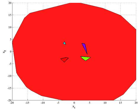
The relaxation is far from good, despite the reasonable variable bounds. This is just a general feature of big-M models. To obtain better models, better bounds are required. Here, we can easily generate this by finding a bounding box of the union, by solving four bounding box problems (note that this requires the solution of 422 linear programs)

[~,L1,U1] = boundingbox(A1*x <= b1);
[~,L2,U2] = boundingbox(A2*x <= b2);
[~,L3,U3] = boundingbox(A3*x <= b3);
[~,L4,U4] = boundingbox(A4*x <= b4);
L = min([L1 L2 L3 L4],[],2);
U = max([U1 U2 U3 U4],[],2);
F = [(A1*x <= b1) | (A2*x <= b2) | (A3*x <= b3) | (A4*x <= b4)];
F = [F, L <= x <= U];

plot(F,x,[],500,sdpsettings('relax',1))
hold on
plot(A1*x<=b1)
plot(A2*x<=b2)
plot(A3*x<=b3)
plot(A4*x<=b4)

Analyzing your model to derive good bounds on all variables involved in expressions ending up in big-M reformulations is a central part of the modelling task.

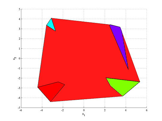
Convex hulls

The goal in a big-M model is to create a model whose relaxation is as close as possible to the convex hull of the original constraint, i.e. the best possible convex approximation of the original feasible set. Clearly, from the figures above, this was not successful. In many cases, good variable bounds lead to reasonably good approximations of the convex hull, and for some models, the convex hull will be recovered.

It is possible to directly generate the convex hull in YALMIP, by using the command hull.

F = hull(A1*x <= b1,A2*x <= b2,A3*x <= b3,A4*x <= b4)
clf
plot(F,x)
hold on
plot(A1*x<=b1)
plot(A2*x<=b2)
plot(A3*x<=b3)
plot(A4*x<=b4)

With this construction, we can create a much stronger mixed integer model of our original model.

M1 = 50;
M2 = 50;
M3 = 50;
M4 = 50;
F = sum(d) == 1;
F = [F, A1*x - b1 <= M1*(1-d(1))];
F = [F, A2*x - b2 <= M2*(1-d(2))];
F = [F, A3*x - b3 <= M3*(1-d(3))];
F = [F, A4*x - b4 <= M4*(1-d(4))];
F = [F, hull(A1*x <= b1,A2*x <= b2,A3*x <= b3,A4*x <= b4)];

The big-M part ensures the equivalence with the original model, while the convex hull part ensures that the integer relaxations are of good quality. Note that the convex hull part introduces many more variables and constraints.

Alternatively, and much more efficient, is to catch the second output from hull and constrain these to be binary. By doing so, a complete mixed-integer convex hull based model is defined easily.

[F,t] = hull(A1*x <= b1,A2*x <= b2,A3*x <= b3,A4*x <= b4);
clf
plot(F,[],[],500);
hold on;
plot([F,binary(t)]);