Envelope approximations for global optimization

The global solver BMIBNB is a YALMIP-based implementation of a standard spatial branch-and-bound strategy. If you are unfamiliar with the basic ideas in a branch & bound solver, you should try to find an introduction first and then perhaps check out the article on global optimization

A branch & bound solver

A spatial branch & bound algorithm for nonconvex programming typically relies on a few standard steps.

1. The starting open node is the original optimization problem constrained to a box which outerbounds the feasible space.

2. In an open node, a local nonlinear solver is applied and may find a feasible (and hopefully locally optimal) solution. This gives an upper bound on the achievable objective (possibly infinite if the solver fails to find a feasible solution). The local solver for this step is specified with the option ‘bmibnb.uppersolver’ in BMIBNB.

3. As a second step a convex relaxation of the model in the node is derived (using the methods described below), and the resulting convex optimization problem is solved (typically a linear program, or if the original problem is a nonconvex semidefinite program, a semidefinite program, or perhaps a convex quadratic or second-order cone problem, depending on what convex relaxation we have). This gives a lower bound on the achievable objective in this box. The lower bound solver is specified using the options ‘bmibnb.lowersolver’ in BMIBNB. If the lower bound is larger than the best upper bound so far, the node can be discarded as the optimal solution cannnot be located in this box.

4. Given these lower and upper bounds, if the node was not discarded a standard branch-and-bound logic is used to select a branch variable, a branch point, divide current box into two new boxes and create the two resulting nodes, branch, prune and navigate among the remaining nodes in a tree of open nodes using (2).

In addition to these standard steps, a large amount of preprocessing and bound-propagation is performed, both in the root-node and along the branching. This is extremely important in order to obtain stronger linear relaxations as we will see below. Some options controlling this can be found in the description of BMIBNB.

Convex envelope approximations

The central object in the solver is the relaxation model which is derived once bounds are available in a node, and this model is built using outer approximations of convex envelopes (the convex hull of the set \( (x,f(x)) \) on some interval in \(x\)).

Linear relaxation for bilinear and quadratic problems

The solver implements a standard relaxation strategy where all bilinear and quadratic terms are replaced with new linear variables. Based on bounds on the variables in the term, constraints are added to relate the new linear variable with the original nonlinear term, in order to make the relaxation as tight as possible.

Given two variables \(x\) and \(y\), and lower and upper bounds \(x_L\), \(x_U\), \(y_L\), \(y_U\), the following inequalities trivially hold McCormick 1976

A linear relaxation of the nonlinear monomials is obtained by introducing new variables \(w_x\), \(w_{xy}\) and \(w_y\), and replacing \(x^2\), \(xy\) and \(y^2\) in the constraints above and the original model with these \(w\) variables. This procedure is applied to all nonlinear terms. A set of linear inequalities (and equalities if there are any) is then obtained outer bounding the original model.

We can use YALMIP to illustrate this for a simple scalar nonlinearity \(x^2\). We create the nonlinear representation of the generating inequalities

sdpvar x;
xL = -1;
xU = 2;
constraints =[(xU-x)*(x-xL)>=0,(xU-x)*(xU-x)>=0,(x-xL)*(x-xL)>=0]

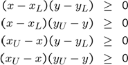
A linear relaxation is obtained by introducing a new variable, and using this variable instead of \(x^2\). This is what happens when you use the option relax when you solve an optimization problems. Any monomial term is treated as an independent variable. We can use this options also when plotting, hence easily showing the linear relaxation.

plot(constraints,[x;x^2],[],[],sdpsettings('relax',1))
t = (-1:0.01:2);
hold on;plot(t,t.^2);

The horizontal axis is the original variable \(x\) and the vertical is the relaxed variable representing \(x^2\), and the polytope shows the feasible region for the relaxed variable. The approximation is tight at the bounds, but fairly poor in the middle. Non-negativity on variables representing quadratic terms are automatically appended in the envelope implementation, thus cutting off the lower negative portion of the polytope (see below)

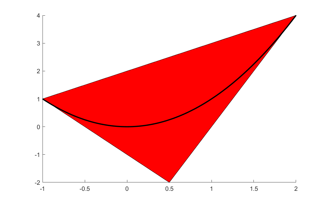
By tightening the bounds during the branching process, the linear relaxation will become increasingly better in nodes down the tree. As an example, if the solver branches on \(x\) at 0.5, two new nodes would be created with stronger relaxations.

sdpvar x;
xL1 = -1;
xU1 = 0.5;
xL2 = 0.5;
xU2 = 2;

constraints1 =[(xU1-x)*(x-xL1)>=0,(xU1-x)*(xU1-x)>=0,(x-xL1)*(x-xL1)>=0]
constraints2 =[(xU2-x)*(x-xL2)>=0,(xU2-x)*(xU2-x)>=0,(x-xL2)*(x-xL2)>=0]

clf
plot(constraints1,[x;x^2],[],[],sdpsettings('relax',1))
hold on
plot(constraints2,[x;x^2],[],[],sdpsettings('relax',1))
t = (-1:0.01:2);
hold on;plot(t,t.^2);

Note that the machinery requires bounds on the variables. BMIBNB extracts all explicit bounds in the model in the root-node and applies several tricks to improve these, and find implied bounds on variables for which no bounds have been supplied. Still, you should always add as much information as possible, and possibly artificial bounds. The tighter the bounds are, i.e., closer to the final optimal value, the better the envelope approximations will be, and the faster the global solver will converge.

Linear relaxation for multivariate polynomial problems

Multivariate polynomial problems are treated by simply converting them to bilinear representions by introducing additional variables and constraints. As an example, the term \(x^2y^2\) can be written as \(uv\) with the new bilinear equality constraints \(u=x^2\) and \(v=y^2\). Once a bilinear model has been obtained, standard bilinear relaxations can be used on the three monomials \(x^2, y^2, uv\).

Linear relaxation for univariate higher degree monomials

Higher degree monomials can be either be handled by applying same idea as for multivariate terms, or by using the general envelope approximation methods described below. BMIBNB applies both strategies depending on context.

Linear relaxation for general univariate operators

A nonlinear scalar term \(f(x)\) is replaced with a new variable \(w\), and linear inequalities on \(x\) and \(w\) are introduced to ensure that \(w\) approximates \(f(x)\) well, i.e., that the curve \(w = f(x)\) is contained in the polytopic region in \(A_x x + A_w w \leq b\).

For this to work, every operator (exp, sin, coth…) has to be apply to supply the envelope polytope data \((A,b)\) given bounds \(x_L\) and \(x_U\). Indeed, this is supported in the infrastructure in YALMIP which is based on operator overloading. Not only does an operator know what it should evaluate to, but it can be equipped with a lot of extra knowledge.

The engine in YALMIP allows every operator to announce properties which can be used by, e.g., BMIBNB. The most common important properties and methods are

• f(x) The function value
• derivative(x) Derivative at x
• inverse(x) Function inverse x
• convexhull(xL,xU) Polytope data \(A,b\) for outer approximation of convex hull
• domain() Domain for the function
• bounds(xL,xU) Local information about function range (lower and upper bounds) in an interval
• vexity() Global convexity information (‘convex’,’concave’,’none’)
• vexity(xL,xU) Local convexity information in interval (‘convex’,’concave’,’none’)
• monotonicity() Global information about monotonicity (‘increasing’, ‘decreasing’, ‘none’)
• monotonicity(xL,xU) Local information about monotonicity in interval (‘increasing’, ‘decreasing’, ‘none’)
• definiteness() Global information about monotonicity (‘negative’, ‘positive’, ‘none’)
• definiteness(xL,xU) Local information about monotonicity in interval (‘negative’, ‘positive’, ‘none’)
• range() Global information about range of function (lower and upper)
• inflection() Information about where function switches convexity , and in what direction
• stationary() Points where the function is stationary
• singular() Points where the function is singular

The important property for us is convexhull(xL,xU) (although we soon will see that this is almost never used).

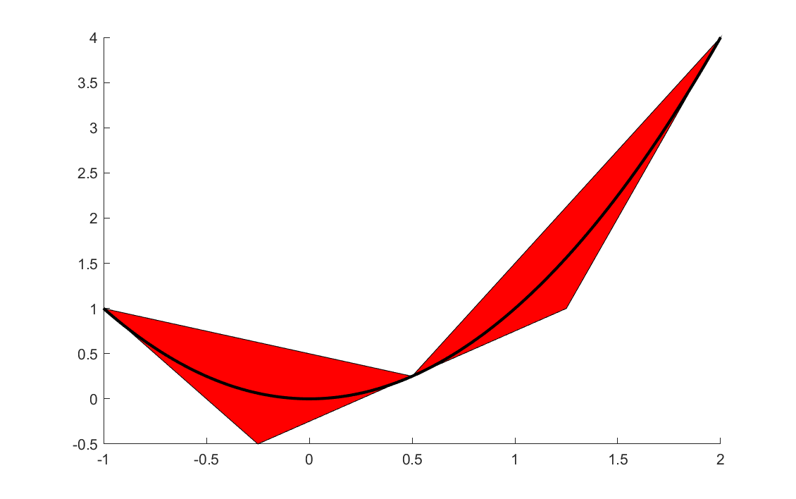
As an example, let us create an outer approximation of the convex hull for sqrtm which is the standard nonlinear overloading of \(\sqrt{x}\). The function is concave, and this means that a convex hull approximation can be constructed by two upper tangent hyperplanes in the end-points, and a lower hyperplane connecting the function values in the two end-points.

xL = 0.1;
xU = 3;
Aw = [1; 1; -1];
xM = (xL + xU)/2;
b = [sqrt(xL) - xL/(2*sqrt(xL));
     sqrt(xU) - xU/(2*sqrt(xU));
     sqrt(xU)*(xL)/(xU-xL) -  sqrt(xL)*(xU)/(xU-xL)];

Ax = [-1/sqrt(4*xL);
      -1/sqrt(4*xU);
       sqrt(xU)/(xU-xL) - sqrt(xL)/(xU-xL)];
sdpvar x w
figure
plot([Ax*x + Aw*w <= b],[x;w]);
t = (xL:0.01:xU);
hold on;plot(t,sqrt(t));

Luckily, manual implementation of code like this is not needed in many places inside YALMIP. Instead, BMIBNB can check if the operator exports a derivative method, and if the function claims to be convex or concave on the interval automatically generate the outer approximation using tangent planes etc.

The operator information is exploited as much as possible. If both a convex hull generator and explicit convexity information is missing, but the operators returns information about inflection points, this can be used to see if the function is convex or concave on the interval and generate a convex hull approximation accordingly. In the case of the quadratic function above, we saw the need of adding a additional cut to avoid the negative region, and this is done automatically using information about the range of the function.

In the absolute worst-case scenario where no information is supplied, and nothing is known, a sampling strategy is used to derive the linear relaxation. This would essentially only be the case if a user has added an operator without supplying any properties or tailor-made convex hull generator. To illustrate a sampling based approximant, the following code computes an approximation of the convex envelope of sin using three facets.

xL = 0;
xU = 3*pi/2;
z = linspace(xL,xU,100);
fz = sin(z);
k1 = max((fz(2:end)-fz(1))./(z(2:end)-xL))+1e-3;
k2 = min((fz(2:end)-fz(1))./(z(2:end)-xL))-1e-3;
k3 = min((fz(1:end-1)-fz(end))./(z(1:end-1)-xU))+1e-3;
k4 = max((fz(1:end-1)-fz(end))./(z(1:end-1)-xU))-1e-3;
Ax = [-k1;k2;-k3;k4];
Aw = [1;-1;1;-1];
b =  [k1*(-z(1)) + fz(1);-(k2*(-z(1)) + fz(1));k3*(-z(end)) + fz(end);-(k4*(-z(end)) + fz(end))];
sdpvar x w
figure
plot([Ax*x + Aw*w <= b],[x;w]);
t = (xL:0.01:xU);
hold on;plot(t,sin(t));

Exploiting YALMIPs internal framework

In the code above, we generated the envelope approximations manually, but it is possible to hook into the inner workings of YALMIP to study these sets.

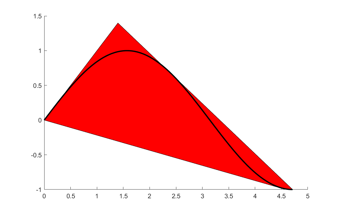
Our sin example

clf
sdpvar w x
E = envelope([0 <= x <= 3*pi/2, w == sin(x)]);
plot(E,[x;w],[],[],sdpsettings('relax',1));
hold on
x = linspace(0,3*pi/2,100);
plot(x,sin(x))

Note that the envelope object E still contains the sin(x) variable (in practice it can be eliminated and replaced with w, but for implementation purposes it is kept in the form above with a trivial equality in the model), hence we must tell YALMIP to relax all variables, and then plot the projection to the \(x,w\) plane.

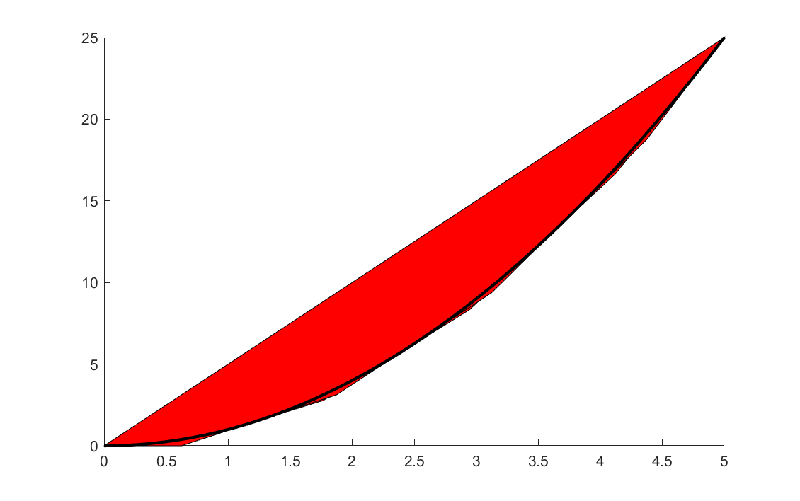
If you study the quadratic monomial from earlier, you will see that YALMIP not only adds a positivity cut to the quadratic envelope, but also adds three tangency cuts. How many cuts BMIBNB uses is basically a trade-off between tightness of the relaxations, and the computational effort needed in the lower bound solvers with additional cuts.

sdpvar w x
E = envelope([0 <= x <= 5, w == x^2]);
plot(E,[x;w],[],[],sdpsettings('relax',1));
hold on
x = linspace(0,5,100);
plot(x,x.^2)

The importance of bounds

Finally, a comment on bounds. As a general rule of thumb, you have to bound all variables used in nonlinear exressions when you use the global solver BMIBNB which is based on envelope approximations. However, YALMIP performs various bound strengthening schemes to improve bounds and find implied bounds, and the same code is used in the envelope code used above. In some cases, YALMIP can derive bounds, without any initial bounds being specified at all. As an example, the following problem is easily solved with nicely behaved envelopes despite supplying no bounds

sdpvar x
optimize([x + x^2 + x^4 == 0],x,sdpsettings('solver','bmibnb'));

YALMIP easily derives the initial bound \(-1 \leq x \leq 0\) and then improves it further to \(-0.6875 \leq x \leq 0\) (the optimal solution is \(x=-0.6823\), so the lower bound is essentially tight), and can use this when creating the cuts for the envelope approximation. A bit silly plot, but you will get a line in \(x\) here showing the feasible interval.

E = envelope([x + x^2 + x^4 == w, w == 0]);
plot(E,[x;w],[],[],sdpsettings('relax',1));

Can you also derive the interval from the nonlinear equation?