Sparse parameterizations in optimizer objects
Notice that the core in YALMIP has had some performance improvements which makes the use of an optimizer object less beneficial in this example. Nevertheless, the general idea introduced here with a sparse parameterization in the optimizer is still important.
The optimizer framework can be used to reduce overhead significantly when solving many similiar problems, by pre-compiling a model parameterized in set of parameters which can change.
The goal with optimizer is to move as much as possible of YALMIP overhead related to model analysis, solver selection, operator modelling, and extraction of low-level numerical models closer to solver formats, to a pre-compilation stage, and then only adjust a small part of the partially compiled model when some parameter changes, before compiling the final solver model and sending it to the solver.
However, with a complicated parameterization, such as when the parameter enters the model nonlinearly with decision variables (bilinear being the typical case, as below), this still requires rather complicated symbolic manipulations when forming the final model given a parameter value.
In the following model, we are going to study a case where we intend to solve a large ampount of non-negativity constrained least-squares problems \( \min_{x\geq 0} \left\lVert Ax - b\right\rVert \), with the particular feature that all data matrices \(A\), which will be a parameter, has a known sparse banded structure.
Let us begin by defining a test-case
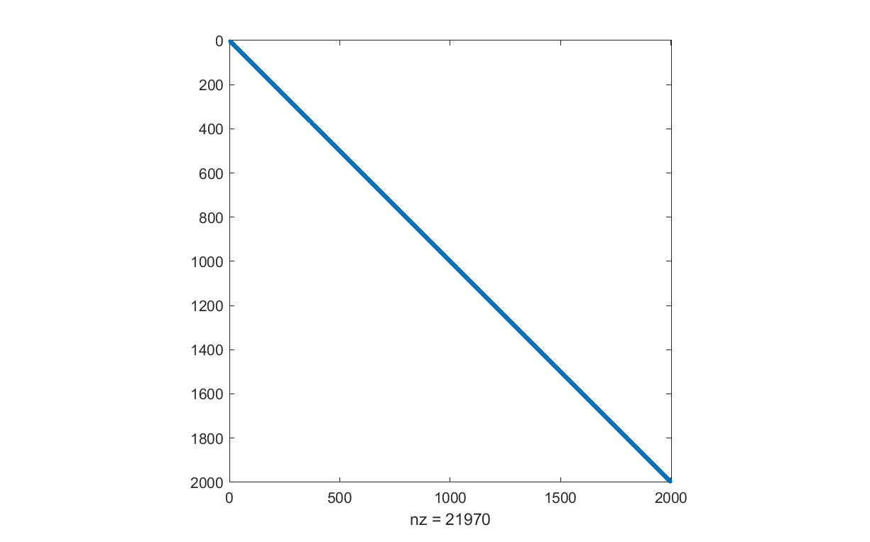
n = 2000;
% Very sparse banded data matrix
Ad = triu(tril(randn(n),5),-5);
bd = randn(n,1);
spy(Ad)
If we only want to solve one single instance, the code is trivial. We use and explicitly specify Mosek here, but you can of course use any SOCP solver you want. Note that a non-negativity constrained least-squares problem also can be formulated as a quadratic program by squaring the objective, but we want to keep it in SOCP form as we want the model to be linearly parameterized in \(A\) and \(b\).
x = sdpvar(n,1);
optimize(x >= 0, norm(Ad*x - bd),sdpsettings('solver','mosek'))
We note that it takes YALMIP more time to analyze the problem, select solver, and create the numerical model for the solver, as it takes for the solver to solve the problem. Actually, this problem is so easy that you have to turn off the display to time the solver accurately, as most time is spent in printing in the MATLAB command window
optimize(x >= 0, norm(Ad*x - bd),sdpsettings('solver','mosek','verbose',0))
This is not an issue if we only want to solve 1 problem, but what if we want to solve 1000 problems for different data with the same structure?
To get rid of the analysis and numerical model extraction overhead when solving many problems of this type, we update our code and try to make a parameterized object which (we think…) will allow us to rapidly solve the problem for varying data,. Let’s test this on our single instance (don’t run this if you are in a hurry!)
A = sdpvar(n,n,'full');
b = sdpvar(n,1);
Solver = optimizer(x >= 0, norm(A*x - b)),sdpsettings('solver','mosek'),{A,b},x);

xd = Solver(Ad,bd);
Unfortunately, this will be a massively complicated object. The expression Ax involves 4 million symbolic monomials and it takes around 10 minutes to just create that expression! This is perhaps not a major issue if we can win back that time when we solve our problems, but we will meet more problems. Creating the solver object once Ax is formed takes another minute or so, but also this is a one-time occurance. However, once we start using the solver object, it’s even more problematic. It turns out that the call with a data instance takes 5 minutes!, i.e., horribly slow compared to setting up the model from scratch.
The problem is the extremely complicated bilinear object. When we send data to the solver object, it has to reason over and manipulate that massive 4 million terms object, in order to reduce the symbolic terms by replacing parameters with given data.
However, since we know that most of the elements in the data matrices are zero, there is no reason to introduce a symbolic data matrix which is fully parameterized. Instead, we should only parameterize the terms which actually can become non-zero. Luckily, the optimizer object supports this sparsity reduced parameterization. All data matrices will have the same sparsity pattern as our test case, hence we can use it to zero out all elements in A which never will be anything but 0 anyway. Note that we do a yalmip(‘clear’) to clear out all internal stuff generated when we created our massive symbolic object above
yalmip('clear')
x = sdpvar(n,1);
b = sdpvar(n,1);
A = sdpvar(n,n,'full');
A = A.*(Ad ~= 0);
Solver = optimizer(x >= 0, norm(A*x - b),sdpsettings('solver','mosek'),{A,b},x);

tic
xd = Solver(Ad,bd);
toc
The optimizer object is now created in roughly 30 seconds, but most importantly every use of the optimizer object only takes around 0.3 seconds, meaning that the overhead has been significanty reduced compared to the fully parameterized model. There is still significant overhead though as we know the solver only needs around 0.1 seconds, but this comes from the fact that the symbolic model still is very large. For n=1000, the overhead is drastically reduced and the optimizer call and the total time is 0.1 seconds of which 0.05 seconds is spent in solver, and for n = 500 the total time is 0.04 seconds with 0.02 seconds spent in solver. Note that for the case n = 500, there are still close to 6000 symbolic terms in the precompiled object, so the fact that there is remaining overhead is not surprsing.
