Linear programming

In this example, we are given two sets of data, called blues and greens. Our goal is to separate these sets using a linear classifier.

blues = randn(2,25);
greens = randn(2,25)+2;

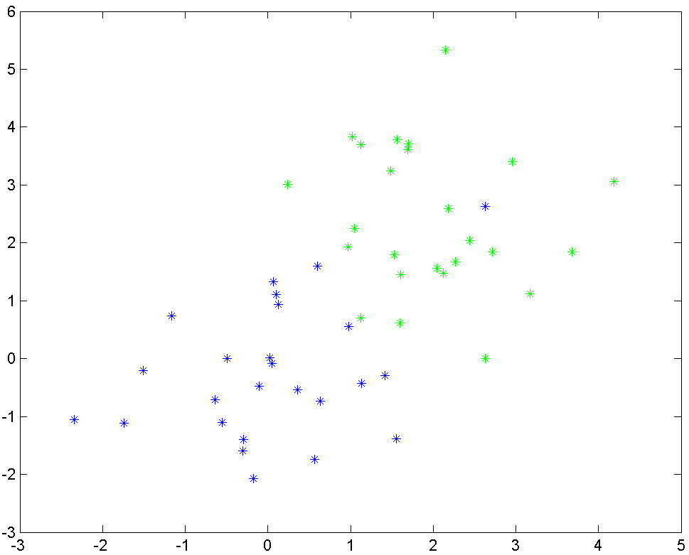
Display the two clusters of data.

plot(greens(1,:),greens(2,:),'g*')
hold on
plot(blues(1,:),blues(2,:),'b*')

A linear classifier means we want to find a vector \(a\) and scalar \(b\) such that \(a^Tx + b \geq 0\) for all the green points, and \(a^Tx+b\leq 0\) for all blue points (a separating hyperplane). By looking at the data, it should be clear that this is impossible. What one then would like to do, is to find a hyperplane which misclassifies as few points as possible. This is typically a very hard combinatorial problem, so we will work with an approximation instead.

As a proxy for misclassification, we introduce positive numbers \(u\) and \(v\) and change the classification to \(a^Tx+b\geq 1-u\) and \(a^Tx+b\leq -(1-v)\). If both \(u\) and \(v\) are small, we should obtain a good separation.

We define the decision variables of interest

a = sdpvar(2,1);
b = sdpvar(1);

We will use one \(u\) and \(v\) variable for each point, hence we create two vectors of suitable length. It will be obvious below why we define them as row-vectors.

u = sdpvar(1,25);
v = sdpvar(1,25);

The classification constraints are easily defined by exploiting MATLABs and YALMIPs ability to add scalars and vectors

Constraints = [a'*greens+b >= 1-u, a'*blues+b <= -(1-v), u >= 0, v >= 0]

We want \(u\) and \(v\) to be small, in some sense, as that indicates a good classification. A simple choice is to minimize the sum of all elements \(u\) and \(v\). However, the problem is ill-conditioned in that form, so we add the constraint that the absolute value of all elements in \(a\) are smaller than \(1\).

Objective = sum(u)+sum(v)
Constraints = [Constraints, -1 <= a <= 1];

Absolute value is convex and LP-representable, so we could just as well have used the built-in command abs, but here we build the LP as basic as possible.

At last, we are ready to solve the problem

optimize(Constraints,Objective)

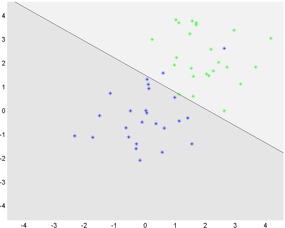
The values of the optimal \(a\) and \(b\) are obtained using value. To better illustrate the results, we use YALMIPs ability to plot constraint sets to lazily display the separating hyperplane.

x = sdpvar(2,1);
P1 = [-5<=x<=5, value(a)'*x+value(b)>=0];
P2 = [-5<=x<=5, value(a)'*x+value(b)<=0];
clf
plot(P1);hold on
plot(P2);
plot(greens(1,:),greens(2,:),'g*')
plot(blues(1,:),blues(2,:),'b*')