Second order cone programming

Let us continue with our regression problem from the quadratic programming tutorial

Robust regression

The problem boiled down to solving the problem minimize \(\left\lVert y - A\hat{x}\right\rVert \) for some suitable norm. Let us select the 2-norm, but this time solve the extension where we minimize the worst-case cost, under the assumption that the matrix \(A\) is uncertain, \(A=A+d\), where \(\left\lVert d\right\rVert_2 \leq 1 \) . This can be shown to be equivalent to minimizing \(\left\lVert y - A\hat{x} \right\rVert_2 \) + \(\left\lVert y - A\hat{x} \right\rVert_2 \).

This problem can easily be solved using YALMIP. Begin by defining the data where we not only have noise in the measurements \(y\) but also a corrpution in the regressors

x = [1 2 3 4 5 6]';
t = (0:0.02:2*pi)';
Atrue = [sin(t) sin(2*t) sin(3*t) sin(4*t) sin(5*t) sin(6*t)];
ytrue = Atrue*x;
A = Atrue;
A(100:210,:)=.1;
y = ytrue+randn(length(ytrue),1);

As a first approach, we will do the modelling by hand, by adding second-order cones using the low-level command cone.

xhat = sdpvar(6,1);
sdpvar u v

F = [cone(y-A*xhat,u), cone(xhat,v)];
optimize(F,u + v);

By using the automatic modelling support in the nonlinear operator framework, we can alternatively write it in the following epigraph form

xhat = sdpvar(6,1);
sdpvar u v

F = [norm(y-A*xhat,2) <= u, norm(xhat,2) <= v];
optimize(F,u + v);

Of course, we can write it in the most natural form (and YALMIP will automatically perform the epigraph reformulation and represent the model using second-order cone operators)

optimize([],norm(y-A*xhat,2) + norm(xhat,2));

YALMIP will automatically model this as a second-order cone problem, and solve it as such if a second-order cone programming solver is installed. If no second-order cone programming solver is found, YALMIP will convert the model to a semidefinite program and solve it using any installed semidefinite programming solver.

Evaluation

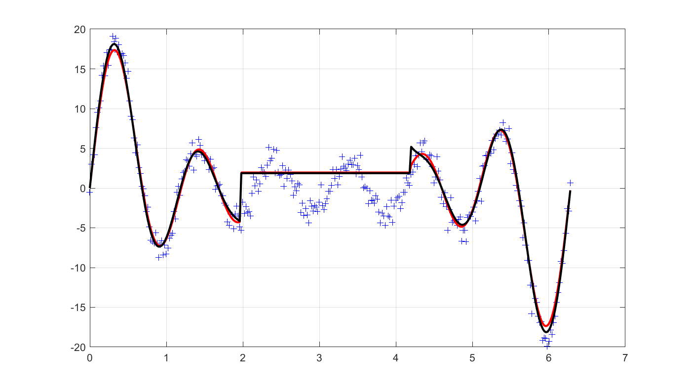
Let us plot the solution, and then see what standard least-squares would have obtained. Note that this is the performance on the real regressor. Our regularization has protected us from over-fitting too much to the corrupt data.

clf
plot(t,y,'+b');
hold on
plot(t,Atrue*value(xhat),'r');
grid on

optimize([],norm(y-A*xhat,2));
plot(t,Atrue*value(xhat),'k');

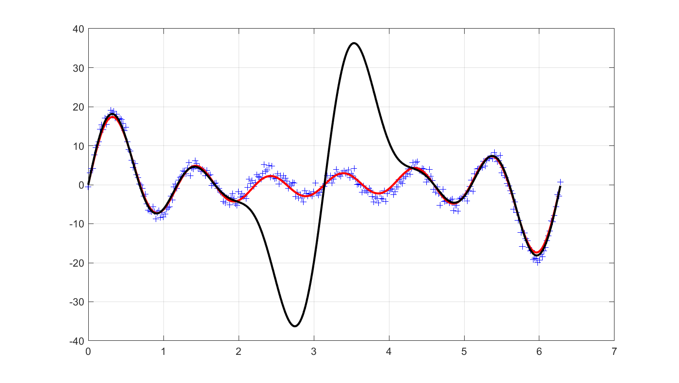
Interestingly, the result on the given corrupt training data is essentially the same.

clf
plot(t,y,'+b');
hold on
optimize([],norm(y-A*xhat,2) + norm(xhat,2));
plot(t,A*value(xhat),'r');
grid on

optimize([],norm(y-A*xhat,2));
plot(t,A*value(xhat),'k');