Quadratic programming

A slight generalization from linear programming leads us to quadratic programming, here focusing on the convex case. Non-convex quadratic programming is possible too, but it is orders of magnitudes harder and a much more complex problem.

Typical applications of convex quadratic programming are variants of least-squares estimation.

Regression

Let us assume that we have data generated from a noisy linear regression \(y_t = a_tx + e_t\). The goal is to estimate the parameter \(x\), given the measurements \(y_t\) and \(a_t\), and we will try 3 different approaches based on linear and quadratic programming.

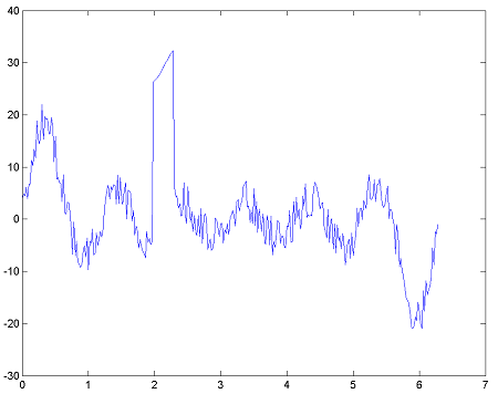
Create some noisy data with severe outliers to work with.

x = [1 2 3 4 5 6]';
t = (0:0.02:2*pi)';
A = [sin(t) sin(2*t) sin(3*t) sin(4*t) sin(5*t) sin(6*t)];
e = (-4+8*rand(length(t),1));
e(100:115) = 30;
y = A*x+e;
plot(t,y);

Define the variable we are looking for

xhat = sdpvar(6,1);

Linear programming regression

By using \( \hat{x}\) and the regressors, we can define the residuals \( e = y - A\hat{x}\) (which also will be an sdpvar object, parametrized in the sought variable \(\hat{x}\))

e = y-A*xhat;

To solve the 1-norm regression problem (minimize sum of absolute values of residuals), we can define a variable that will serve as a bound on the absolute values of \(e\) (we will solve this problem much more conveniently below by simply using the norm operator)

bound = sdpvar(length(e),1);

Express that the bound variables are larger than the absolute values of the residuals (note the convenient definition of a double-sided constraint).

Constraints = [-bound <= e <= bound];

Call YALMIP to minimize the sum of the bounds subject to the constraints modelling the abolsute values. YALMIP will automatically detect that this is a linear program, and call any LP solver available on your path.

optimize(Constraints,sum(bound));

The optimal value is, as always, extracted using the overloaded value command.

x_L1 = value(xhat);

Minimize the \(\infty\)-norm. This corresponds to minimizing the largest (absolute value) residual. Introduce a scalar to bound the largest value in the vector residual (YALMIP uses MATLAB standard to compare scalars, vectors and matrices)

bound = sdpvar(1,1);
Constraints  = [-bound <= e <= bound];

and minimize the bound.

optimize(Constraints,bound);
x_Linf = value(xhat);

Quadratic programming regression

The 2-norm problem (least-squares) is easily solved as a QP problem without any constraints.

optimize([],e'*e);
x_L2 = value(xhat);

YALMIP automatically detects that the objective is a convex quadratic function, and solves the problem using any installed QP solver. If no QP solver is found, the problem is converted to an SOCP, and if no dedicated SOCP solver exist, the SOCP is converted to an SDP (although at that point you are better of explicitly telling YALMIP via sdpsettings to use a standard nonlinear solver, which will be much better than using an SDP solver).

With quadratic programming, we typically mean linear constraints and quadratic objective, so let us solve such a general problem by adding a 1-norm regularization to our least-squares estimate.

bound = sdpvar(length(e),1);
Constraints = [-bound <= e <= bound];
optimize(Constraints,e'*e + sum(bound));

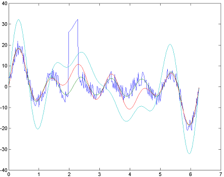
We plot the solutions, and notice that the 1-norm estimate worked very well and essentially managed to capture the underlying harmonics despite the severe measurement error after 2 seconds, whereas the other estimates perform badly on this data set.

plot(t,[y A*x_L1 A*x_L2 A*x_Linf]);

Note that the low-level manipulations here can be performed much easier by using the nonlinear operator framework in YALMIP.

optimize([],norm(e,1));
optimize([],norm(e,inf));
optimize([],e'*e + norm(e,1));

Large-scale quadratic programs

The 2-norm solution (least-squares estimate) is most classically stated in the described QP formulation, although it in some cases is much more efficient in YALMIP to express the problem using a 2-norm, which will lead to a second-order cone problem.

optimize([],norm(residuals,2));

The reason is that a quadratic function with \(n\) variables can be composed of up to \(n(n+1)/2\) monomials, which YALMIP has to work with symbolically. If you absolutely need to solve a large-scale quadratic program with YALMIP using a QP solver, introduce an auxiliary variable and equality constraints. This will make the quadratic term sparse and move any dense data to the linear equality constraints (not only YALMIP but many QP solvers will be significantly faster after this transformation)

s = sdpvar(length(e),1);
optimize([s == e],s'*s);

Of course, in this example, it makes no difference, as there only are 6 decision variables but in scenarios where your objective is \(x^TQx\) and \(Q=R^TR\) is large and dense, a better model might be

R = chol(Q);
s = sdpvar(length(x),1);
optimize([s == R*x],s'*s);

Even better, if you know \(Q\) is low-rank or there is some other structure that allows you to compute a low-rank possibly sparse factor, you should exploit that

R = my_smart_factorization(Q);
s = sdpvar(size(R,2),1);
optimize([s == R*x],s'*s);

The archetypical example is sum(x)^2 which leads to a completely dense quadratic model of rank 1. Absolutely catastrophical for large problems (it will most likely be indefinite for vectors of length larger than 10 in floating-point numerics) and a waste of memory. The trivial improvement is

s = sdpvar(1);
optimize([s == sum(x)],s^2);

Finally, note that squaring a 2-norm expression simply returns the quadratic function, i.e., the following two calls are equivalent and no SOCP modelling is performed. In other words, the introduction of a possibly complicated symbolic quadratic object is not circumvented here.

optimize([],norm(R*e)^2);
optimize([],e'*R'*R*e);