Multiparametric programming

This tutorial requires MPT.

YALMIP can be used to calculate explicit solutions of parametric linear and quadratic programs by interfacing the Multi-Parametric Toolbox MPT. This tutorial assumes that the reader is familiar with parametric programming and the basics of MPT.

Generic example.

Consider the following simple quadratic program in the decision variable z, solved for a particular value on a parameter x.

A = randn(15,3);
b = rand(15,1);
E = randn(15,2);

z = sdpvar(3,1);
x = [0.1;0.2];

F = [A*z <= b+E*x];
obj = (z-1)'*(z-1);

sol = optimize(F,obj);
value(z)
ans =
   -0.1454
   -0.1789
   -0.0388

To obtain the parametric solution with respect to x, we call the function solvemp, and tell the solver that x is a parametric variable. Moreover, we must add constraints on x to define the region where we want to compute the parametric solution, the so called exploration set.

x = sdpvar(2,1);
F = [A*z <= b+E*x, -1 <= x <= 1];
sol = solvemp(F,obj,[],x);

The first output is an MPT structure. In accordance with MPT syntax, the optimizer for the parametric value (0.1,0.2) is given by the following code.

xx = [0.1;0.2];
[i,j] = isinside(sol{1}.Pn,xx)
sol{1}.Fi{j}*xx + sol{1}.Gi{j}
ans =
   -0.1454
   -0.1789
   -0.0388

By using more outputs from solvemp, it is possible to simplify things considerably.

[sol,diagnostics,aux,Valuefunction,OptimalSolution] = solvemp(F,obj,[],x);

The function now returns solutions using YALMIPs nonlinear operator framework. To retrieve the numerical solution for a particular parameter value, simply use assign and value in standard fashion.

assign(x,[0.1;0.2]);
value(OptimalSolution)

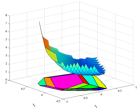
Some of the plotting capabilities of MPT are overloaded for the piecewise functions. Hence, we can plot the piecewise quadratic value function

plot(Valuefunction);

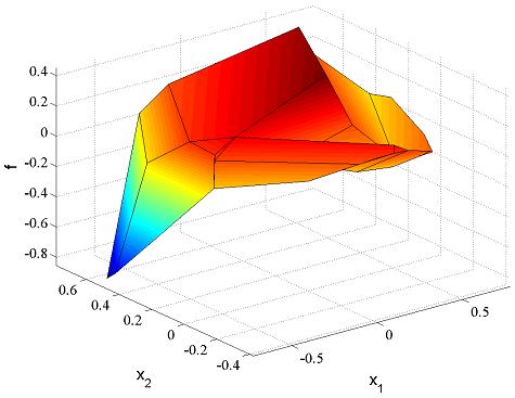
and plot the piecewise affine optimizer

figure
plot(OptimalSolution(1));

Simple MPC example

Define numerical data for a linear system \(x_{k+1} = Ax_k + Bu_k, y_k = Cx_k\), and variables for state \(x\), and control sequence \( u\), for an MPC problem with horizon 5.

A = [2 -1;1 0];
B = [1;0];
C = [0.5 0.5];
x = sdpvar(2,N+1,'full');
u = sdpvar(1,N);

Create the MPC predictions, with input and state constraints, in a so called explicit form where we optimize over both inputs and states, with a cost quadratic in the output and input.

Objective = 0;
Model = [];
for i = 1:N
    Objective = Objective + x(:,i+1)'*C'*C*x(:,i+1) + u(i)^2;
    Model = [Model, x(:,i+1) == A*x(:,i) + B*u(i)];
    Model = [Model, -1 <= u(i) <= 1, -5 <= x(:,i+1) <= 5];
end

Add a constraint on the initial state which will serve as a definition of the exploration set for the parametric program.

Model = [Model, -5 <= x(:,1) <= 5];

We are ready to use solvemp to solve the multi-parametric program in the initial state, and we ask for the parametric solution for the first input.

[sol,diagnostics,aux,Valuefunction,OptimalSolution] = solvemp(F,objective,[],x(:,1),u(1));

We can plot the overloaded solutions directly

figure
plot(Valuefunction)
figure
plot(OptimalSolution)

Mixed integer multiparametric programming

YALMIP extends the multiparametric solvers in MPT by adding support for binary variables in the parametric problems.

We will now solve this problem under the additional constraints that the input is quantized in steps of 1/3. This can easily be modelled in YALMIP using ismember. Note that this nonconvex operator introduces a lot of binary variables, and the MPC problem is most likely solved more efficiently using a dynamic programming approach. Since the input at every time instant can take 7 different values, it means a brute-force approach to computing the multi-parametric solution will in the worst-case require solution of \(7^N\) multi-parametric programs. Unfortunately, that is lmost what happens here, so we reduce the horizon to 3.

N = 3;
x = sdpvar(2,N+1,'full');
u = sdpvar(1,N);
Model = [];
Objective = 0;
for i = 1:N
    Objective = Objective + x(:,i+1)'*C'*C*x(:,i+1) + u(i)^2;    
    Model = [Model, x(:,i+1) == A*x(:,i) + B*u(i)];
    Model = [Model, -1 <= u(i) <= 1, -5 <= x(:,i+1) <= 5];
    Model = [Model, ismember(u(i),[-1:1/3:1])];
end
Model = [Model, -5 <= x(:,1) <= 5];

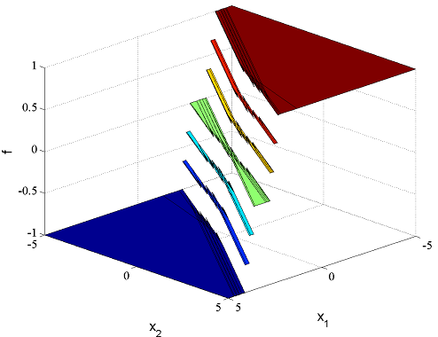
Same commands as before to solve the problem and plot the optimal solution

[sol,diagnostics,aux,Valuefunction,OptimalSolution] = solvemp(F,objective,[],x(:,1),u(1));
plot(OptimalSolution);

For more examples, see the dynamic programming example, the robust MPC example, the portfolio example, and the MAXPLUS control example.