Semidefinite programming
This example illustrates the definition and solution of a simple semidefinite programming problem.
Given a linear dynamic system \(\dot{x} = Ax\), our goal is to prove stability by finding a symmetric matrix \(P\) satisfying
\[\begin{align}A^TP + PA &\prec 0\\P &\succ 0\end{align}\]Define a stable matrix \(A\) and symmetric matrix \(P\) (remember: square matrices are symmetric by default)
A = [-1 2 0;-3 -4 1;0 0 -2];
P = sdpvar(3,3);
Having defined \(P\), we are ready to define the semidefinite constraints.
F = [P >= 0, A'*P+P*A <= 0];
Note that we have defined non-strict inequalities, although our theoretical problem involves strict inequalities. YALMIP will warn or submit and error if you use strict inequalities.
Strict inequalities simply does not make much sense in continuous numerical optimization.
If you want to satisfy a strict inequality, you have to define a non-strict inequality with a margin.
To avoid the zero solution on this homogeneous problem we can for instance add a margin and use \(P \succeq I \) (which additionally ensures we obtain a strictly feasible solution), or as we do here, constrain the trace of the matrix to dehomogenize the solution.
F = [F, trace(P) == 1];
At this point, we are ready to solve our problem. But first, we display the collection of constraints to see what we have defined.
F
+++++++++++++++++++++++++++++++++++
|   ID|                 Constraint|
+++++++++++++++++++++++++++++++++++
|   #1|      Matrix inequality 3x3|
|   #2|      Matrix inequality 3x3|
|   #3|    Equality constraint 1x1|
+++++++++++++++++++++++++++++++++++
We only need a feasible solution, so one argument is sufficient when we call optimize to solve the problem.
optimize(F);
Pfeasible = value(P);
The resulting constraint satisfaction is easily investigated with check.
check(F)
++++++++++++++++++++++++++++++++++++++++++++++++++++++++++++++++++
|   ID|            Constraint|   Primal residual|   Dual residual|
++++++++++++++++++++++++++++++++++++++++++++++++++++++++++++++++++
|   #1|     Matrix inequality|           0.20138|     8.2785e-016|
|   #2|     Matrix inequality|            1.1397|     3.6687e-016|
|   #3|   Equality constraint|       -2.276e-015|    -8.1801e-016|
++++++++++++++++++++++++++++++++++++++++++++++++++++++++++++++++++
Minimizing, e.g., the top-left element of \(P\) is done by specifying an objective function.
F = [P >= 0, A'*P+P*A <= 0, trace(P)==1];
optimize(F,P(1,1));
We can easily add additional linear inequality constraints. If we want to add the constraint that all off-diagonal elements are larger than zero, one approach is (remember, standard MATLAB indexing applies)
F = [P >= 0, A'*P+P*A <= 0, trace(P)==1, P([2 3 6])>=0];
optimize(F,P(1,1));
Since the variable P([2 3 6]) is a vector, the constraint is interpreted as a standard linear inequality, according to the rules introduced in the basic tutorial.
Finally, let us solve a robust stabilization problem to show how we can use for-loops
A = [-1 2 0;-3 -4 1;0 0 -2];
P = sdpvar(3,3);
F = [P >= eye(3)]
for i = 1:20
    Ai = A + rand(3);
    F = [F, Ai'*P+P*Ai <= 0];
end
optimize(F,trace(P));
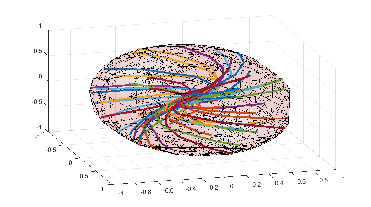
The computed matrix \(P\) defines an invariant ellipsoid, so let us lot trajectories to see that this really holds true
P = value(P);
clf
x = sdpvar(3,1);
plot(x'*P*x <= 1,x,[],[],sdpsettings('plot.shade',.1));

hold on
for i = 1:30
    Ai = A + rand(3);
    f = @(t,x)(Ai*x);
    x0 = randn(3,1);x0 = x0/sqrt((x0'*P*x0));
    X = ode45(f,[0 20],x0);
    l = plot3(X.y(1,:),X.y(2,:),X.y(3,:));
    set(l,'Linewidth',3);drawnow
end