Exponential cone programming
The exponential cone is defined as the set \( (ye^{x/y}\leq z, y>0) \), see, e.g. Chandrasekara and Shah 2016 for a primer on exponential cone programming and the equivalent framework of relative entropy programming. YALMIP is capable of detecting and calling specialized solvers for a variety of exponential cone representable functions.
By simple variable transformations, the following functions are automatically detected as exponential cone representable and suitably rewritten before calling an exponential cone capable solver
Note that YALMIP does not necessarily automatically detect exponential cones when written in the canonical form \( ye^{x/y}\leq z \), but instead you can use the perspective exponential, pexp, which implements \( ye^{x/y} \).
A low-level approach to define exponential cones is the command expcone.
The code below is primarily intended for solvers with dedicated exponential cone support which currently is Mosek, SCS or ECOS. However, YALMIP also supports the exponential cone operator expcone and exponential cone representable functions such as logsumexp which is used below in general nonlinear solvers such as fmincon. When a general nonlinear solver is used, exponential cone representable functions are used in their native form and not converted to an exponential cone representations.
Logistic regression example
As an example, we solve a logistic regression problem. The problem here is to find a classifier \( \operatorname{sign}(a^Tx + b)\) for a given dataset \( x_i\) with associated labels \( y_i = \pm 1 \). In other words, a classifier similiar to the simple separating hyperplane discussed in the linear programming tutorial.
A convex relaxation of the problem can be solved by minimizing \( \sum \log(1 + e^{-y_i(a^Tx_i + b)}) \). This can be written as a sum of logsumexp operators by noting that \( \log(1 + e^{z})=\log(e^{0} + e^{z}) \). In YALMIP, you do not have to think further, but can use the logsumexp operator directly to solve the problem. However, let us show how this boils down to a simple exponential cone program.
To begin with, the problem can be written as minimizing \( \sum t_i \) subject to \( \log (e^0 + e^{-y_i(a^Tx_i + b)}) \leq t_i \). The constraint is first rewritten by exponentiating both sides to \(e^0 + e^{-y_i(a^Tx_i + b)} \leq e^{t_i} \), which is equivalent to \(e^{-t_i} + e^{-y_i(a^Tx_i + b)-t_i} \leq 1 \), which can be further normalized to \(z_i + u_i \leq 1, e^{-t_i}\leq z_i, e^{-y_i(a^Tx_i + b)-t_i} \leq u_i\), which thus lands us in a standard exponential cone program.
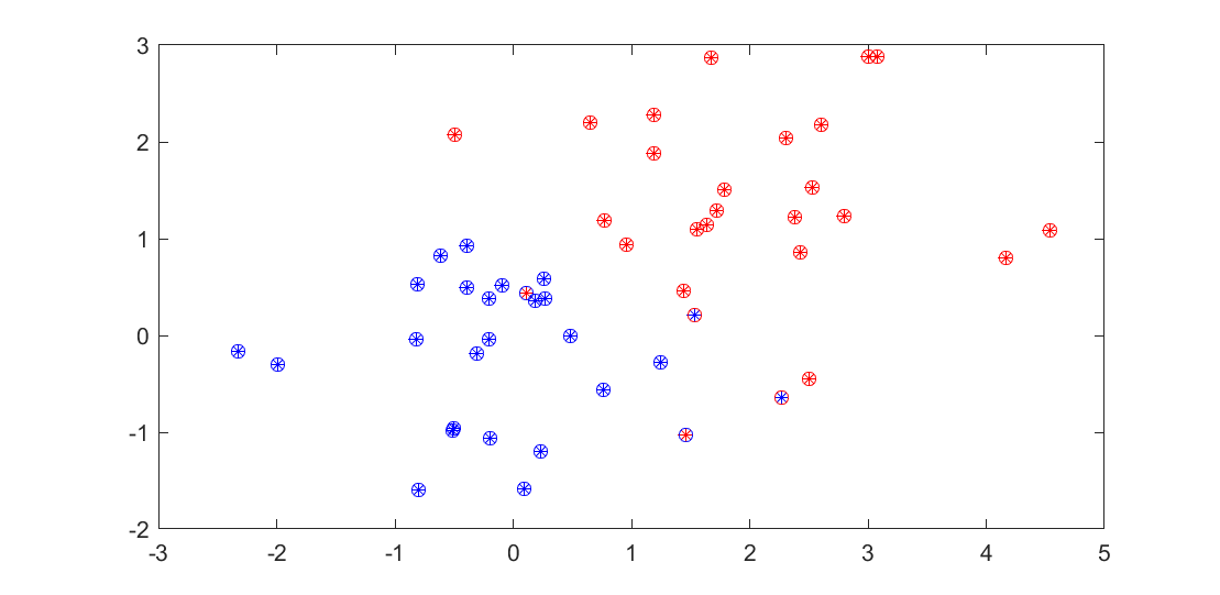
Generate data as in the linear programming tutorial for a classification problem.
N = 50;
blues = randn(2,N/2);
reds = randn(2,N/2)+2;
clf
plot(reds(1,:),reds(2,:),'r*');hold on
plot(blues(1,:),blues(2,:),'b*')
Solve the problem using the built-in logsumexp operator which automatically models the problem as an exponential cone program if an exponential cone program solver is specified. Note that logsumexp applied to a matrix will return a vector with logsumexp applied to every row. If you have an exponential cone programming solver installed, it will automatically be selected.
% blue = 1, red = -1
x = [blues reds];
y = [repmat(1,1,length(blues)) repmat(-1,1,length(reds))];

a = sdpvar(2,1);
b = sdpvar(1);
J = sum(logsumexp([zeros(length(y),1) (-y.*(a'*x + b))']'))
optimize([],J);
We study the result by marking the data points with a ring colored according to the computed classifier, and count the number of mis-classified training points
class = sign(value(a'*x+b));
classB = find(class == 1);
classR = find(class == -1);
plot(x(1,classB),x(2,classB),'bo')
plot(x(1,classR),x(2,classR),'ro')
nnz(sign(value(a'*x+b))-y)
Of course, nothing forces us to use linear separators
X = [x;x(1,:).^2;x(2,:).^2;x(1,:).*x(2,:)]
a = sdpvar(size(X,1),1);
b = sdpvar(1);
J = sum(logsumexp([(-y.*(a'*X + b))' zeros(length(y),1)]'))
optimize([],J);
class = sign(value(a'*X+b));
classB = find(class == 1);
classR = find(class == -1);
plot(x(1,classB),x(2,classB),'bo')
plot(x(1,classR),x(2,classR),'ro')
nnz(sign(value(a'*X+b))-y)
Comments
If the exponential cone program violates convexity rules, and an exponential cone solver is selected an error will be issued
sdpvar x
optimize([],log(x), sdpsettings('solver',scs'))
