Power cone programming

The power cone as we use it is defined as the set \( \left \lvert z \right\rvert_2 \leq x^{\alpha}y^{1-\alpha}, x\geq 0, y\geq 0 \) for constant \( 0 < \alpha < 1\). In contrast to exponential cones, YALMIP does not detect and reformulate models to power cones. Instead, power cones can only be used as a low-level construct via pcone, with a small exception illustrated below.

The code below requires Mosek 9 as this is the only power cone solver available in YALMIP.

Geometric example

The following example called the p-norm geometric median of a point cloud is taken from Moseks power cone introduction. Given a set of points \(x_i\) our task is to find the point \(y\) minimizing \( \sum_i \left \lvert y-x_i \right\rvert_p \) for different \(p > 1\). We use the power cone representation from Mosek and show how it is implemented using pcone. Afterwards, we also use a built-in command pnorm which implements a power cone representation of the p-norm.

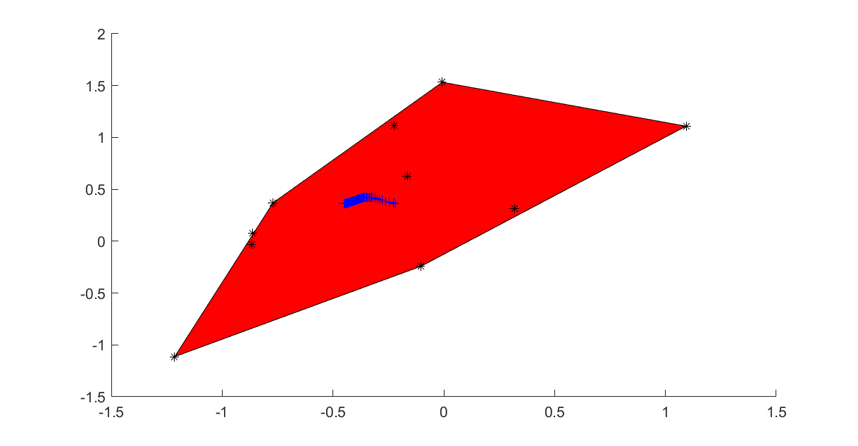
Generate some random points, and plot them together with the convex hull

n = 10;
x = randn(2,n);
s = sdpvar(n,1);
z = sdpvar(2,1);
clf;
plot([z == x*s, s>=0, sum(s)==1],z);hold on
plot(x(1,:),x(2,:),'k*');

Low-level approach via pcone

We start with a low-level scalar implementation of the sum of p-norms, and we trace the solution as a function of \(p\).

t = sdpvar(1,n);
r = sdpvar(2,n);
y = sdpvar(2,1);
objective = sum(t);
for p = 1.1:0.1:10
    Model = [sum(r) == t];
    for i = 1:2
        for j = 1:n
            Model = [Model, pcone(r(i,j),t(j),y(i) - x(i,j),1/p)];        
        end
    end
    optimize(Model,objective)
    plot(value(y(1)),value(y(2)),'b+')
    drawnow
end

A vectorization over the samples can be made to make the code more compact (the vectorization could of course be performed also over the dimension, but we leave it here as we only want to illustrate that multiple power cones can be created with one command)

t = sdpvar(1,n);
r = sdpvar(2,n);
y = sdpvar(2,1);
objective = sum(t);
for p = 1.1:0.1:10
    Model = [sum(r) == t];
    for i = 1:2        
      Model = [Model, pcone([r(i,:);
                             t;
                             y(i)-x(i,:);
                             repmat(1/p,1,n)])];
    end
    optimize(Model,objective)
    plot(value(y(1)),value(y(2)),'y+')
    drawnow
end

High-level code via pnorm

Power cones are currently only supported via the low-level pcone operator, and the only high-level use of power cones is that the p-norm representation used above is available in the command pnorm. By default it is implemented using a second-order cone representation, so a third argument is needed.

for p = 1.1:0.1:10
    objective = 0;
    for j = 1:n
        objective = objective + pnorm(y-x(:,j),p,'power');        
    end
    optimize([],objective)
    plot(value(y(1)),value(y(2)),'g+')
    drawnow
end