Experiment design in system identification

This article accompanies the paper Wernholt and Löfberg 2007.

The problem has its origin in an optimal experiment design problem for identification of physical parameters of an industrial robot with significant nonlinear and flexible behaviour.

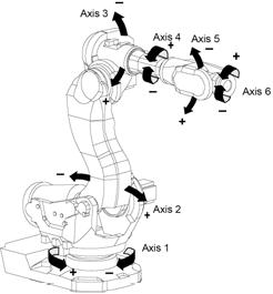
In order to estimate physical parameters, identification experiments can be performed with the robot positioned in various configurations (angles of the robot links). By discretizing the possible positions, a large number of candidate positions are defined, and with each position, an associated covariance matrix is computed. This covariance matrix is a lower bound on the achievable estimation performance that can be obtained by performing an identification experiment locally around this position.

The problem is to combine these covariance matrices from different positions to achieve a minimal combined covariance matrix. This can be interpreted as computing the number of experiments performed in each configuration.

To define an optimal covariance matrix, a scalar measure on the matrix has to be introduced. In the paper, the minimum volume confidence ellipsoid was used, also called D-optimal design. This can be written as minimization of the determinant of the inverse combined covariance matrix.

Combinatorial D-optimal design

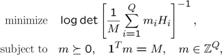
Let \(Q\) denote the total number of possible configurations and \(H_i\) the 12-by-12 inverse covariance matrices from each configuration. Our goal is to perform \(M\) experiments. The D-optimal design problem can be written as

This problem can be solved using YALMIPs internal mixed integer conic solver BNB. Due to the logdet term, you are advised to solve the problem using SDPT as the lower bound solver.

Load the covdata.mat and use straightforward code to define the combined covariance matrix. Since this problem is combinatorial, we have to resort to a small number of candidates, compared to the problems we will solve below. Hence, we let Q=200 and M=15.

urlwrite('https://raw.githubusercontent.com/yalmip/yalmip.github.io/master/pub/covdata.mat', 'covdata.mat');
load covdata
Q = 200;
M = 15;
m = intvar(Q,1);
H = 0;for i = 1:Q;H = H + m(i)*Hi{i};end

Minimizing the logarithm of the determinant of the inverse of the covariance matrix is equivalent to maximizing the logarithm of the determinant of the covariance matrix. The problem is solved in a couple of seconds.

constraints = [m>= 0, sum(m)==M];
objective = -logdet(H);
options = sdpsettings('solver','bnb','bnb.solver','sdpt3');
optimize(constraints, objective, options);

Although the combinatorial D-optimal design problem can be solved using YALMIP for reasonably small \(Q\), the paper focus on the relaxed problem, since a much larger \(Q\) was used in the application.

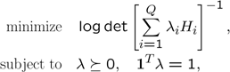
Relaxed problem in original form

A relaxed problem is obtained by simply skipping the integrality constraint. When the integrality constraint is removed, the problem can be thought of as finding the time ratio spent in each configuration. For that purpose, a normalized problem is solved.

We now solve a larger problem using this initial form of the problem. First, to speed up the construction of the \(H\) matrix, we vectorize the code.

Q = 1000;
lambda = sdpvar(Q,1);
Hvec = reshape([Hi{:}],12^2,[]);
H = reshape(Hvec(:,1:Q)*lambda,12,12);

The problem is solved in a couple of seconds. In case you have alternative SDP solvers on your path, the code explicitly selects sdpt3 to ensure that the logdet is treated in the most efficient way.

constraints = [lambda >= 0, sum(lambda ) == 1];
objective = -logdet(H);
options = sdpsettings('solver','sdpt3');
optimize(constraints, objective, options);

Although the code is capable of solving medium-sized problems, sdpt3 (and any other SDP solver) will run into memory problems when \(Q\) goes beyond a couple of thousands.

However, with some knowledge on how SDP problems are solved, this low limit on tractable problems comes as a surprise. The problem, when stated as above, is actually a very small SDP problem, also for large \(Q\). However, it is only a small problem when interpreted in a primal sense. Unfortunately, YALMIP always interpret problems in a dual sense. To understand the following section, you are advised to have a look at the automatic dualization tutorial

Relaxed problem in dualized form

Since the optimization problem is small when interpreted in a primal sense, but YALMIP always interprets problems in a dual sense, we can trick YALMIP by deriving and stating the dual problem instead.

Manual derivation of the dual problem leads to the following determinant maximization problem (\(d\) denotes the dimension of the \(H\) matrix).

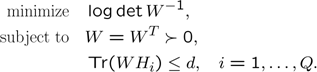
Whereas the original problem had \(Q\) variables when interpreted in a dual sense, the new problem only has 78 variables (the variables needed to parametrize the 12-by-12 symmetric matrix \(W\). The large amount of variables in the original problem now leads to a large amount of linear inequalities. However, complexity with respect to the number of linear inequalities in the dual, is much better than complexity with respect to the number of variables.

We solve the new problem, and notice that it is solved much faster. Once again we vectorize the code to speed up the YALMIP code.

W = sdpvar(12,12);
constraints = [Hvec'*W(:) <= 12];
objective = -logdet(W);
options = sdpsettings('solver','sdpt3');
optimize(constraints, objective, options);

The original variables can be recovered from the duals associated to the linear inequality constraints.

dual(constraints)

Manually deriving the dual problem is cumbersome, and problematic for most users. Luckily, the [automatic dualization] feature in YALMIP can do this automatically, and keep track of variables. Simply state the original problem, and tell YALMIP to derive the dual, solve the problem, and recover the original variables.

The dualized form is much more efficient, and allows us to solve the complete problem, which for the data here is Q=7920.

Q = 7920;
lambda = sdpvar(Q,1);
Hvec = reshape([Hi{:}],12^2,[]);
H = reshape(Hvec(:,1:Q)*lambda,12,12);

constraints = [lambda >= 0, sum(lambda ) == 1];
objective = -logdet(H);
options = sdpsettings('solver','sdpt3','dualize',1);
optimize(constraints, objective, options);

If you study the output displayed by sdpt3 you will see that the solver reports that there are 79 variables. In the manual model, a scalar term in the objective function was explicitly minimized and removed from the problem. Interestingly, sdpt3 behaves better numerically on the automatically generated dual problem than the manually derived model.