Star-convex polygons

This example currently only runs on the develop branch

In the grey area between convex and non-convex sets, there is a geometry which is called star-convex (star-domain, star-shaped, radially convex). As the name reveals, a classical drawing of a star is a special case.

Mathematically, the definition of a (origin-centered) star-convex set is that all points between the origin and any point in the set is in the set. Compare this to the definition of a convex set where all points on a line between any two points are in the set. Loosely speaking, it is convex w.r.t a particular point (here the origin). The origin can be changed to some other so called vantage point by translating the whole set and defining star-convexity w.r.t the translated origin.

Here, we will play around with star-convex polygons, modelling them both manually and by using built-in support.

Note that you need a sos2 capable solver such as GUROBI or CPLEX.

Star-convex polygons

Define some data representing the vertices of a star (remember, a star-convex set does not have to look like a star, it is just a name)

n = 6;
th = linspace(-pi, pi, 2*n+1);
xi = (1+rem((1:2*n+1),2)).*cos(th);
yi = (1+rem((1:2*n+1),2)).*sin(th);
clf;
hold on;
grid on
plot( xi, yi, 'b*-' );
axis equal;

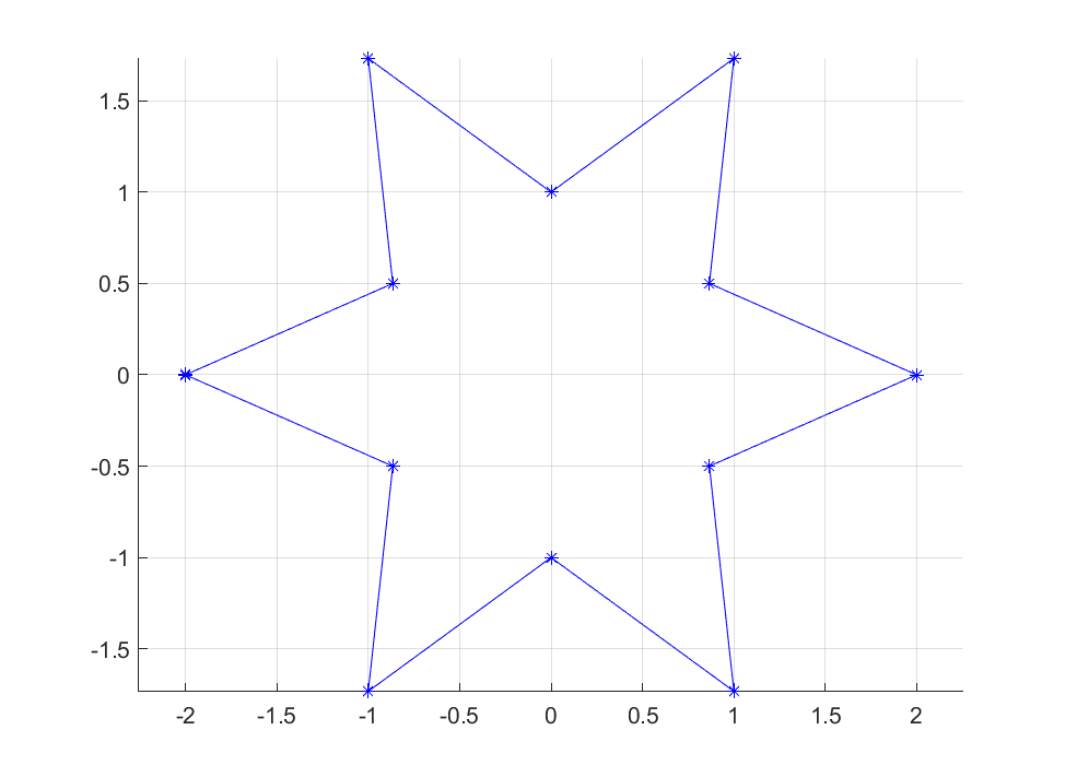
Note that we have generated the coordinates so that they represent a closed curve, i.e. the first and last values are the same. This is important to remember when you create these sets using the methods described here.

The feasible set inside the star can be represented as the union of 7 polytopes. Hence, a general approach to representing this set is to describe these polytopes, and then use logic programming and binary variables to represent the union as illustrated in the big-M tutorial. However, star-convex polygons can be represented much more conveniently using sos2 constructs.

To derive a sos2 representation, we first focus on representing the border of the polygon. With given vertices \(v_i = (x_i,y_i)\), every point on the border of the star can be written as a linear combination of two adjacent vertices. This can be written as \(V\lambda\) where where \(V\) are the vertices stacked in columns and \(\lambda\) is a non-negative vector with at most two adjacent non-zero elements summing up to \( 1\). This is the classical application of sos2, and precisely the same model YALMIP uses for linear interpolation in interp1 which essentially is what we are doing here.

Assuming we work with coordinates \(x\) and \(y\) as decision variables in our model, and we want to say that \((x,y)\) is on the border, we arrive at the model

sdpvar x y
lambda = sdpvar(length(xi),1)
Model = [sos2(lambda), lambda>=0, sum(lambda)==1,
         x == xi*lambda, y == yi*lambda];

That’s all!

To see that this really models what we want, we could plot the set. When doing so, you will note that it is not drawing the star, but the convex hull of the star.

plot(Model,[x;y],[],[],sdpsettings('plot.shade',.1))    

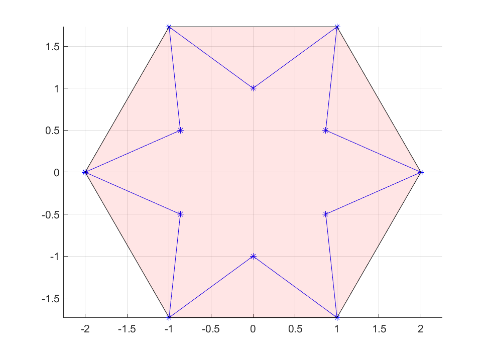
This is not due to an incorrect model, but simply a limitation of the plot command. When you plot a set, it performs ray-shooting to find points on the boundary, and then draws the convex hull of these points (the only way to draw non-convex sets in YALMIP is to explicitly model mixed-integer models, as YALMIP then will perform enumeration of all combinatorial combinations of binry variables and draw each set individually to depict the union)

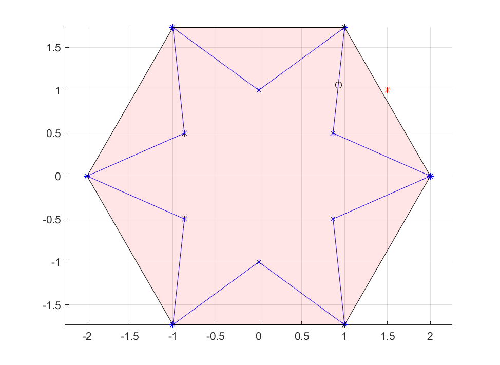
To make sure we actually have modelled the border of the star, let us solve a simple problem where we find the point closest to a point outside.

optimize(Model, (x-1.5)^2 + (y-1)^2)
plot(1.5,1,'*r')
plot(value(x),value(y),'ok')

Scaling and translating

So how can we include the interior? This is where star-convexity comes into play. Since the interior corresponds to all scaled border points, it means we can scale the interpolating \(\lambda\)-variables with an arbitrary scale \(0 \leq t \leq 1\). It also means we can take the adjacent interpolated vertices and scale them individually first, and then interpolate between them. Effectively, this means we can generate the model with

sdpvar x y
lambda = sdpvar(length(xi),1)
Model = [sos2(lambda), lambda>=0,sum(lambda)<=1,
         x == xi*lambda, y == yi*lambda];

This model can be extended further by allowing an arbitrary scaling of the set by using any upper bound on the sum, even a decision variable as the bound enters affinely.

What about the translations and the more general case of star-convexity w.r.t other vantage points than the origin? Let us start by defining a star centered outside the origin, so that star-convexity w.r.t the origin is violated.

n = 6;
th = linspace(-pi, pi, 2*n+1);
xi = 1+(1+rem((1:2*n+1),2)).*cos(th);
yi = 2+(1+rem((1:2*n+1),2)).*sin(th);
clf;
hold on;
grid on
plot( xi, yi, 'b*-' );
axis equal;

If we define the set using the same code as before, the case which only includes the border will still be valid, but the generalization to include the interior is flawed. As the interpolating \(\lambda\) is allowed to be zero, the origin will be included as a feasible point. The problem is that the set is not star-convex w.r.t the origin and the set we would create using our old code is the union of all stars scaled towards the origin.

No problems though, we shift the origin and define the set as a translated star-convex set. Draw its convex hull as a sanity check. In this particular case, we can shift the origin to a vantage point defined as the mean of the coordinates. Note that the last element is a repetition of the first, so the mean is computed on the unique coordinates.

xc = mean(xi(1:end-1));
yc = mean(yi(1:end-1));
lambda = sdpvar(length(xi),1)
Model = [sos2(lambda), lambda>=0,sum(lambda)<=1,
         x == xc + (xi-xc)*lambda, 
         y == yc + (yi-yc)*lambda];
plot(Model,[x;y],[],[],sdpsettings('plot.shade',.1))   

Note that the using the mean of the coordinates as the vantage point is definitely not something which works in all cases. For highly symmetric objects it does, but in general problem specific insight is needed. As an example, the following set (blue) is star-convex (slide it to the left and it is star-convex wr.t. the origin) but after shifting all coordinates using the mean (red) we see that the set is not star-convex w.r.t the origin.

xi = [1 2 2 3 3 4 4 1 1];
yi = [1 1 5 5 1 1 0 0 1];
clf
hold on;
grid on
plot( xi, yi, 'b*-' );
plot( xi-mean(xc), yi-mean(yc), 'r*--' );
axis equal;

Built-in support

As we have seen, by using sos2 it is straightforward to derive a model, but YALMIP has built-in support for creating these sets even more conveniently. By default it only takes the coordinates and the element intended to be in the set and assumes star-convexity w.r.t to the origin. A fourth argument can be used to translate the set, and there is a fifth option to allow for scaling. With a sixth options, you can ask for YALMIP to automatically shift the model to derive a star-convexity model around a particular point, the mean, median or center of bounding box.

Model = starpolygon(xi,yi,z);       % Define model z in star-convex polygon defined by (xi,yi). Origin assumed to be vantage point
Model = starpolygon(xi,yi,z,c);     % Translate polygon by c (optional)
Model = starpolygon(xi,yi,z,c,t);   % Scale polygon by t (relative vantage point) (optional)
Model = starpolygon(xi,yi,z,c,t,p); % Vantage-point (optional, either a point, or 'mean', median' or 'box')

Construct data for a weird set which is star-convex around (e.g.) \( (1,2) \). Plot the star-convex set and its convex hull (shaded pink), the convex hull of the scaled set (blue), the convex hull of the translated set (yellow), and a scaled version with an alternative vantage point (red).

n = 6;
th = linspace(-pi, pi, 2*n+1);
xi = 1+(1+rem((1:2*n+1),3)).*cos(th).^3;
yi = 2+(1+rem((1:2*n+1),2)).*sin(th);
clf;
hold on;
grid on
plot( xi, yi, 'b*-' );
axis equal;

sdpvar x y
Model = starpolygon(xi,yi,[x;y],[],[],[1;2]);
plot(Model,[x;y],[],[],sdpsettings('plot.shade',.1))    

Model = starpolygon(xi,yi,[x;y],[],.25,[1;2]);
plot(Model,[x;y],'b')  

Model = starpolygon(xi,yi,[x;y],[],0.25,[1;1]);
plot(Model,[x;y],'g') 

Model = starpolygon(xi,yi,[x;y],[-4;0],[],[1;2]);
plot(Model,[x;y],'y')   

Optimizing over star-convex polygons

Let us use our new set and solve some silly optimization problems.

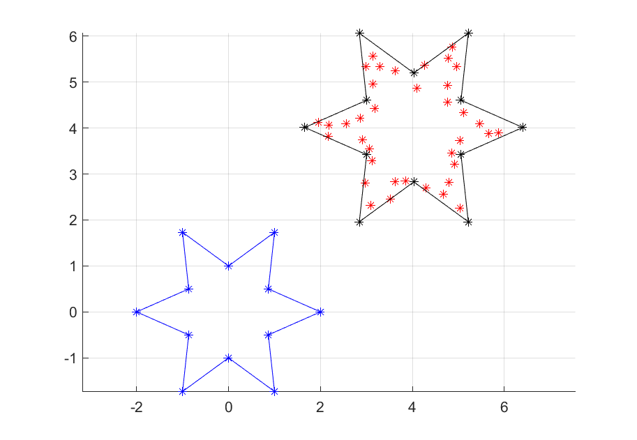
As a first example, we are given a point-cloud (almost looking like a star) and our task is to find the smallest possible star containing all points. We can formulate this as saying that all points in the point-cloud should be in a scaled and translated star, and the goal is to find the optimal translation and scaling.

% Define the template star
n = 6;
th = linspace(-pi, pi, 2*n+1);
xs = (1+rem((1:2*n+1),2)).*cos(th);
ys = (1+rem((1:2*n+1),2)).*sin(th);
clf
hold on;
grid on
plot( xs, ys, 'b*-' );
axis equal;

% Create the point-cloud
thn = linspace(-pi, pi, 2*3*n+1);
xn = 3+interp1(th,xs,thn)+.1*randn(1,2*3*n+1)
yn = 2+interp1(th,ys,thn)+.1*randn(1,2*3*n+1)
plot( xn, yn, 'r*' );

% Now say that each point in point-cloud is in scaled and translated polygon
sdpvar t
c = sdpvar(2,1);
Model = [];
for i = 1:length(xn)
  Model = [Model, starpolygon(xs,ys,[xn(i);yn(i)],c,t)];
end

% Minimize scale factor
optimize(Model,t)

% ...and plot the scaled and translated star
plot( value(t)*xs+value(c(1)), value(t)*ys+value(c(2)), 'k*-' );