Modelling if-else-end statements

YALMIP supports complex models by overloading most standard operators in MATLAB. One common issue though that many users struggle with is models involving if statements. The object-oriented overloading of operators in MATLAB does not support overloading of programming constructs, i.e., if x, elseif x, switch x case y, for x=y where x or y involves sdpvar variables will not work.

Hence, this logic has to be modelled manually, and the recommended approach to do this is to apply the implies operator in a structured fashion.

A nonconvex regression problem

Consider a problem where we wish to do regression \( \textbf{minimize} \sum f(e_i)\) where \(e = y-Ax\) with reduced sensitivity to large outliers by using a non-convex penalty \(f(\cdot)\). Instead of a standard quadratic, linear, or perhaps huber penalty, we want to have a quadratic behaviour for small residuals, linear penalty for medium-sized residuals, and constant penalty for really large residuals. We do not in any sense endorse this regression approach, this is just for illustrating encoding of if statements.

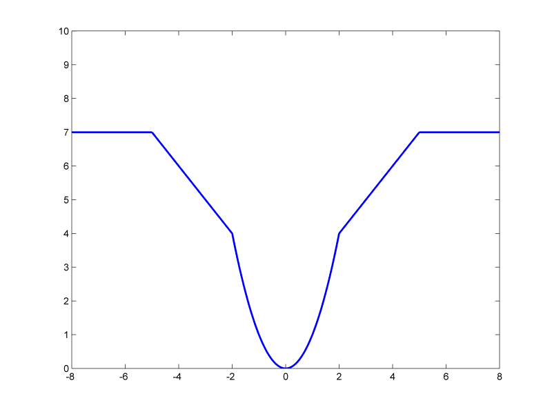
A naive way of formulating this would be \( f(e) = \min(7,\min(2 + \vert x \vert,x^2)) \). However, if you use an objective with a sum of these expressions, the resulting model will be a pretty messy nonconvex integer model. Binary variables will be introduced to handle the fact that the concave \(\min\) operator is used in an expression to be minimized, with more binary variables to handle the nonconvex use of the absolute value, and finally the mixed-integer model will also contain nonconvex quadratic equalities.

A better approach is to try to untangle the model. A first step would be to see it as

This can be simplified even further (note, in optimization simple is not necessarily equivalent to short, but preferably as linear, structured and sparse as possible)

To implement this in MATLAB, we could for instance try to incorporate some code along the lines of

if e <= -5
 f = 7;
elseif e >= -5 && e <= -2
 f = 2-e;
elseif e>=-2 && e <= 2
 f = e^2;
elseif e>=2 && e <= 5
 f = 2+e;
elseif e >= 5 
 f = 7;
end 

This code will not run, and MATLAB will raise an error, as you are you are using an expression involving sdpvar variables in the if construct. What we have to do is to translate this to a simple combinatorial model, and implement that using binary variables.

Enumerate the possible cases

For the cleanest possible code, you should think through what are the possible cases in the most simplified model possible. With simple, we mean no else statements, as few logical combinations as possible, and a set of conditions where only one thing can or should happen. In our case, a list of the possible cases would be

if e <= -5
 f = 2;
end;
 
if e >= -5 && e <= -2
 f = 2-e;
end

if e>=-2 && e <= 2
 f = e^2;
end
 
if e>=2 && e <= 5
 f = 2+e;
end

if e >= 5
 f = 2;
end 

In this case, there are obviously 5 possible cases dividing the feasible space into 5 regions. The strategy now is to introduce 5 binary variables, and create a model where each of these binary variables forces e to be in the associated region, and the corresponding cost function on f to hold. Note that the condition used in the if-statement, and the resulting action, both are moved to a list of constraint.

d = binvar(5,1);
Model = [sum(d) == 1,
implies(d(1), [      e <= -5, f == 7]);
implies(d(2), [-5 <= e <= -2, f == 2-e]);
implies(d(3), [-2 <= e <= 2,  f == e^2]);
implies(d(4), [ 2 <= e <= 5,  f == 2+e]);
implies(d(5), [ 5 <= e,       f == 7])];

At this point, we have a simple cleanly enumerated model, but in this particular case we have a remaining problem as the quadratic equality constraint is nonconvex. However, since we know \(f\) will be minimized, we can relax the equality to a convex inequality. The big-M model that will be derived for implies(d,e^2<=f) would be \(e^2 \leq f + M(1-d)\), which is convex for relaxed integer variables, and hence mixed-integer second-order cone representable. A final proposal is thus

d = binvar(5,1);
Model = [sum(d) == 1,
implies(d(1), [      e <= -5, f == 7]);
implies(d(2), [-5 <= e <= -2, f == 2-e]);
implies(d(3), [-2 <= e <= 2,  f >= e^2]);
implies(d(4), [ 2 <= e <= 5,  f == 2+e]);
implies(d(5), [ 5 <= e,       f == 7])];

Putting it together for a test

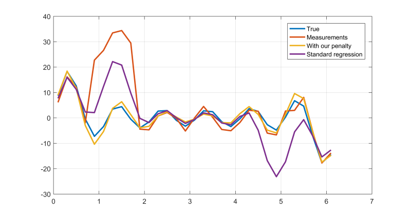
So let us solve the regression problem from the quadratic programming tutorial. We generate some data with non-gaussian noise (we create a considerably smaller problem here, as this combinatorial model is very hard for most solvers)

x = [1 2 3 4 5 6]';
t = (0.1:0.2:2*pi)';
A = [sin(t) sin(2*t) sin(3*t) sin(4*t) sin(5*t) sin(6*t)];
n = (-4+8*rand(length(t),1));
n(5:9) = 30;
y = A*x+n;
plot(t,y);

Define the residuals and function values (which we do in a non-vectorized fashion here). To obtain a sparse structure in the complicated integer constraints, we define e by equalities, instead of making it a dense function of xhat. Note that we have to add explicit bounds on all variables involved in the implications as these are modelled using big-M methods. For the problem to be solved efficiently, you have to have an efficient mixed-integer second order cone programming solver installed. For comparison, we also solve a standard linear regression problem.

xhat = sdpvar(6,1);
f = sdpvar(length(y),1);
e = sdpvar(length(y),1);

xBound = 100;
eBound = norm(y,inf) + norm(A,inf)*xBound;
fBound = max([2 + eBound, 7, eBound^2]);
Model = [          e == y-A*xhat, 
             -xBound <= xhat <= xBound,
             -eBound <= e <= eBound,
             -fBound <= f <= fBound];
      
Objective = sum(f);
for i = 1:length(f)
 d = binvar(5,1);
 Model = [Model, sum(d) == 1,
          implies(d(1), [      e(i) <= -5, f(i) == 7]);
          implies(d(2), [-5 <= e(i) <= -2, f(i) == 2-e(i)]);
          implies(d(3), [-2 <= e(i) <= 2,  f(i) >= e(i)^2]);
          implies(d(4), [ 2 <= e(i) <= 5,  f(i) == 2+e(i)]);
          implies(d(5), [ 5 <= e(i),       f(i) == 7])];
end

optimize(Model,Objective)
xhat1 = value(xhat);
optimize([],e'*e)
xhat2 = value(xhat);
plot(t,[A*x y A*xhat1 A*xhat2]);
legend('True','Measurements','With our penalty','Standard regression')

Converting to quadratic program

As a final note separate from the issues concering if statements, let us try to move from a mixed-integer second-order cone formulation to a mixed-integer quadratic program, which typically can be solved more efficiently. The trick is to realize that the objective either is a linear term, or a squared linear term, depending on where we are. We therefore define each term in the objective as a sum of a linear term and a squared linear term, and zero out suitable parts.

xhat = sdpvar(6,1);
f = sdpvar(length(y),1);
e = sdpvar(length(y),1);

fL = sdpvar(length(y),1);
fQ = sdpvar(length(y),1);

xBound = 100;
eBound = norm(y,inf) + norm(A,inf)*xBound;
Model = [          e == y-A*xhat, 
             -xBound <= xhat <= xBound,
             -eBound <= e <= eBound,
         -(2+eBound) <= fL <= 2 + eBound,
             -eBound <= fQ <= eBound];
      
Objective = sum(fL + fQ.^2);
for i = 1:length(f)
 d = binvar(5,1);
 Model = [Model, sum(d) == 1,
          implies(d(1), [      e(i) <= -5, fL(i) == 7,     fQ(i) == 0]);
          implies(d(2), [-5 <= e(i) <= -2, fL(i) == 2-e(i),fQ(i) == 0]);
          implies(d(3), [-2 <= e(i) <= 2,  fQ(i) == e(i),  fL(i) == 0]);
          implies(d(4), [ 2 <= e(i) <= 5,  fL(i) == 2+e(i),fQ(i) == 0]);
          implies(d(5), [ 5 <= e(i),       fL(i) == 7,     fQ(i) == 0])];

end

optimize(Model,Objective)
xhat1 = value(xhat);
optimize([],(y-A*xhat)'*(y-A*xhat))
xhat2 = value(xhat);
plot(t,[A*x y A*xhat1 A*xhat2]);
legend('True','Measurements','With our penalty','Standard regression')

A more natural model which might lead to problems

It should be said, that a reasonable approach to create a theoretically equivalent model of the logic behaviour is

Model = [implies(      e <= -5, f == 7);
         implies(-5 <= e <= -2, f == 2-x);
         implies(-2 <= e <= 2,  f >= e^2);
         implies( 2 <= e <= 5,  f == 2+x);
         implies(      5 <= e,  f == 7)];

Although this looks much easier, it hides important structure that can cause problems. As all those constraints are added independently, there is nothing in the model which explicitly forces one of the cases to hold. Due to numerical tolerances in solvers, it might be the case that the optimal e ends up at a point on the border between two regions where the solver manages to violate a constraint every so slightly and renders all conditions inactive thus making f undefined. Hence, it is always recommended to explicitly define the disjunctive nature of the model by introducing binary variables which must activate one condition.