Integrating piecewise affine functions

In this example, we will combine methods for expressing if-else statements with built-in support for integrating polynomial functions to develop models involving integrated piecewise affine functions.

Optimizing integrals of piecewise affine functions

Our goal here is to optimize models involving integrals of the form \(\int_0^x f(z)dz \) where \(x\) is a decision variable and \(f\) is a piecewise affine function. Since an integral of an affine function is quadratic, this means we are going to be faced with optimization models involving piecewise quadratic functions.

Let us construct a simple example where our goal is to maximize an integrated piecewise affine function where

An alternative representation is \(\min(\min(4,2z),16-3z)\). To see what we are working with, we plot it and its numerically computed integral.

ti = 0:0.001:10;
fi = min(min(2*ti,4),16-3*ti);
l = plot(ti,fi);
grid on;hold on
l = plot(ti,0.001*cumsum(fi))

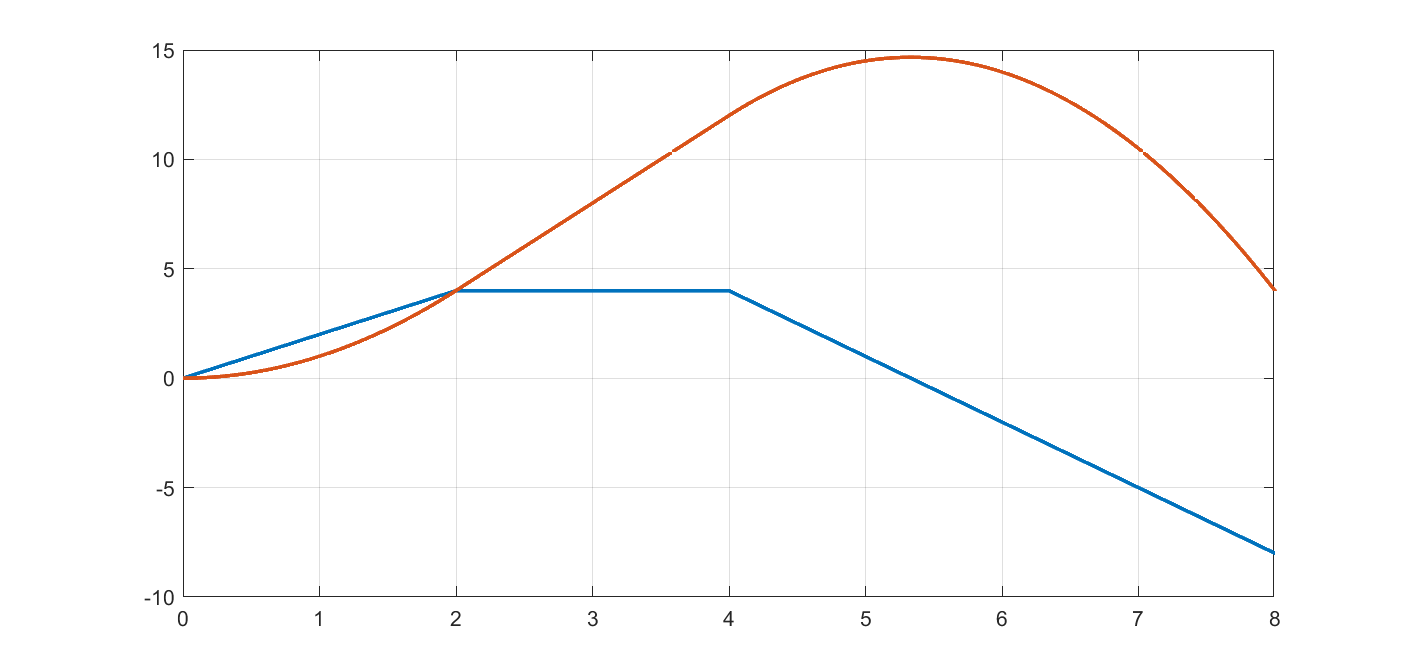
Due to the negative slope in the third region, the piecewise quadratic function is non-convex.

The hard way

As a first approach, we do it the hard way by pen-and-paper computations to explicitly compute the integral to obtain our piecewise quadratic function

Having these expression, we are ready to implement the model. What we have to do is to represent that the objective is defined differently in different regions, which effectively means we have to implement if-else statements. Proceeding exactly as we learn there, we end up with our finished product after having simplified our integrals.

sdpvar x
sdpvar f
region = binvar(3,1);

R1 = [0 <= x <= 2];
R2 = [2 <= x <= 4];
R3 = [4 <= x <= 10];
Model = [implies(region(1), [R1, f == x^2])
         implies(region(2), [R2, f == -4 + 4*x])
         implies(region(3), [R3, f == -28 + 16*x - 1.5*x^2])
         sum(region) == 1
         [0 <= x <= 10, -100 <= f <= 100]];

optimize(Model, -f)

Important to realize is that this model is hard from two different aspects. To begin with, we have binary variables as we have to represent the disjunctive nature, but we also have quadratic equalities inside these disjunctions. Hence, the final product is a mixed-integer nonlinear non-convex quadratically constrained problem. Hence you need a solver such as BMIBNB, GUROBI or BARON.

The even harder but hopefully better way

As we learn in if-else statements, models where a piecewise quadratic function is used in the objective can be improved upon by removing the quadratic equalities from the equalitities and lift them into the objective. The trick to do so is to assign a local copy of the decision variable to each region. Using this strategy here leads to

sdpvar x1 x2 x3
Model = [implies(region(1), [R1, x1 == x, x2 == 0, x3 == 0])
         implies(region(2), [R2, x2 == x, x1 == 0, x3 == 0])
         implies(region(3), [R3, x3 == x, x1 == 0, x2 == 0])
         sum(region) == 1
         [0 <= [x x1 x2 x3] <= 10]];
f = x1^2 + (-4*region(2)+4*x2) + (-28*region(3)+16*x3 - 1.5*x3^2);
optimize(Model, -f)

In this form, we have an MIQP, possibly with nonconvex objective, meaning we are opening up for using CPLEX. Had the piecewise affine functions been non-increasing, the quadratic function would have been concave, and the resulting model here would have had a convex objective, i.e. we would have had a convex MIQP which typically is easier to handle as branching only has to be performed in the combinatorial space, and not in the continuous space. There are more solvers available for this model class too, such as MOSEK. Note though, if we had this convex case, we should really not have modelled the objective using using disjunctions, but written the convex piecewise quadratic function using a convex epigraph representation, leading us to a convex second-order cone program.

Getting lazy

The reason we use YALMIP is because we are lazy, so the models above are too much manual labour. Our goal is to do all the integration related manipulations automatically.

First, note that the integral is \( \int_0^x f(z)dz = \int_0^{u_1} f_1(z)dz + \int_{u_1}^{u_2} f_2(z)dz + \ldots \).

Use int to perform symbolic integration, sum up these parts and we have our piecewise quadratic functions in the three regions.

sdpvar z
sdpvar f
f1 = 2*z; 
f2 = 4;   
f3 = 16-3*z;

q1 = int(f1,z,0,x);
q2 = int(f1,z,0,2) + int(f2,z,2,x);
q3 = int(f1,z,0,2) + int(f2,z,2,4) + int(f3,z,4,x);

The integrals we derived manually seem to be correct

sdisplay(q1)
x^2
sdisplay(q2)
-4+4*x
sdisplay(q3)
-28+16*x-1.5*x^2

We are done and are ready to define the model!

Model = [implies(region(1), [R1, f == q1])
         implies(region(2), [R2, f == q2])
         implies(region(3), [R3, f == q3])
         sum(region) == 1
         [0 <= x <= 10, -100 <= f <= 100]];

optimize(Model, -f)

Can it get any easier than that?

Even lazier

Yes it can.

f = int(f1,z,0,min(x,2)) + int(f2,z,2,min(x,4)) + int(f3,z,4,x);
optimize([0 <= x <= 10], -f)

Too much work?

Crazy lazy

Well then (if you are ok with an approximation).

f = interp1(ti,0.001*cumsum(min(min(2*ti,4),16-3*ti)),x,'sos2');
optimize([0 <= x <= 10],-f)

Leads to a MILP, so no scary nonconvex quadratics.

Just bad

A nonlinear programming representation where the integral is computed on-the-fly during the solution process is obtained with the following.

f = blackbox(@(U)(integral(@(z)(min(min(2*z,4),16-3*z)),0,U)),x);
optimize([0 <= x <= 10],-f);

The use of blackbox means we moved into the territory of completely unstructured nonlinear programming. Not recommended unless the model calls for this due to other complicated parts.