Designing polynomials

In this post, we showcase some of the operations available on polynomials, and illustrate a common polynomial design problem.

We have given the task of designing a polynomial \( p(x) \) such that it satisfies certain properties. To begin with, let us assume the only requirements are the point-wise constraints \( p(x_0) = y_0, p(x_1) \geq y_1\) and \(p(x_2) = y_2\), and we want to design a polynomial of order 9.

Point-wise function values

Start by defining the data in the problem

x0 = -1
x1 = 0;
x2 = 1;
y0 = 0;
y1 = 1;
y2 = 0;
n = 9;

To define polynomials, the most convenients commands are polynomial or possibly monolist. The command polynomial creates a polynomial but also returns the coefficients and the basis

x = sdpvar(1);
[p,a,v] = polynomial(x,n);

The vector \(a\) holds the coefficients, and \(v(x)\) is the corresponding basis in \(p(x) = a^Tv(x)\). To handle point-wise constraints on the polynomial, we use the command replace for evaluation. Solving the initial problem is thus

Model = [replace(p,x,x0)==y0,replace(p,x,x1)>=y1, replace(p,x,x2)==y2];
optimize(Model)

This a trivial linear program in the coefficients \(a\) without any objective. To plot the polynomial, we use built-in functionality (but note that YALMIP has a reveresed order on monomials in a polynomial compared to polyval).

xv = linspace(x0,x2,100);
yv = polyval(fliplr(value(a')),xv);
plot(xv,yv)

Derivatives and integrals

In polynomial design, it is common to have constraints on derivatives in certain points. Since derivatives and integrals of a polynomial are linear operators in the coefficients, we can easily work with these. Hence, let us add the constraint that the polynomial is flat at the end-points, and has non-negative curvature in the middle (for higher order derivatives, simply apply the jacobian command repeatedly)

dp = jacobian(p,x);
dp2 = hessian(p,x);
Model = [replace(p,x,x0)==y0,replace(p,x,x1)>=y1, replace(p,x,x2)==y2,
         replace(dp,x,x0)==0,replace(dp,x,x2)==0,replace(dp2,x,x1)>=0];
optimize(Model)
yv = polyval(fliplr(value(a')),xv);
hold on
plot(xv,yv)

Let us now add an objective. As an example, let us minimize the squared integral \( \int_{-1}^1 p(\tau)^2d\tau\). Note that this is a convex quadratic funtion in \(a\).

Model = [replace(p,x,x0)==y0,replace(p,x,x1)>=y1, replace(p,x,x2)==y2,
         replace(dp,x,x0)==0,replace(dp,x,x2)==0,replace(dp2,x,x1)>=0];
optimize(Model, int(p^2,x,-1,1));
yv = polyval(fliplr(value(a')),xv);
hold on
plot(xv,yv)

Infinite-dimensional constraints

A common situation is that we have infinite-dimensional constraints, i.e., in this context, constraints that should hold for an interval of \(x\), such as positivity or convexity defined by curvature constraints. There are essentially two ways to deal with this, optimistic relaxations based on gridding, and conservative relaxations based on sum-of-squares.

Let us assume we want the polynomial to be non-negative on the interval we are studying. A simple gridding could be something along the lines of

Model = [replace(p,x,x0)==y0,replace(p,x,x1)>=y1, replace(p,x,x2)==y2,
         replace(dp,x,x0)==0,replace(dp,x,x2)==0,replace(dp2,x,x1)>=0];
xgrid = linspace(-1,1,15);     
for i = 1:length(xgrid)
 Model = [Model, replace(p,x,xgrid(i)) >= 0];
end
optimize(Model, int(p^2,x,-1,1));
yv = polyval(fliplr(value(a')),xv);
ygrid = polyval(fliplr(value(a')),xgrid);
hold on
plot(xv,yv);
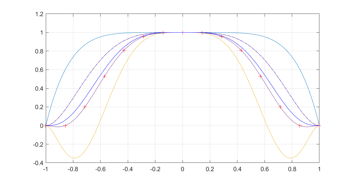
plot(xgrid,ygrid,'r+');
grid on

Unfortunately, with a too coarse gridding, the non-negativity constraint will be violated outside the grid-points.

Instead, we can apply sum-of-squares arguments. We want \(p(x) \geq 0 \) for all \(x^2 \leq 1\). In a sum-of-squares setup, we first rewrite this as finding a certificate polynomial \(s(x)\geq 0\) such that \( p(x) \geq s(x)(1-x^2)\). At this point, the positivity requirements are replaced with sum-of-squares decomposability.

In the following code, we define a parameterised quadratic multiplier \(s(x)\) and solve the sum-of-squares program to find a polynomial \(p(x)\) which is guranteed to be locally non-negative

Model = [replace(p,x,x0)==y0,replace(p,x,x1)>=y1, replace(p,x,x2)==y2,
         replace(dp,x,x0)==0,replace(dp,x,x2)==0,replace(dp2,x,x1)>=0];
[s,c] = polynomial(x,2);
Model = [Model, sos(s), sos(p - s*(1-x^2))];
solvesos(Model, int(p^2,x,-1,1),[],[a;c]);
yv = polyval(fliplr(value(a')),xv);
hold on
plot(xv,yv,'--b');

What you will note though is that the solution is pretty far away from the solution obtained by gridding. The reason is that the method is conservative and the order on the multiplier is too low. By increasing the order, the optimal solution is recovered

Model = [replace(p,x,x0)==y0,replace(p,x,x1)>=y1, replace(p,x,x2)==y2,
         replace(dp,x,x0)==0,replace(dp,x,x2)==0,replace(dp2,x,x1)>=0];
[s,c] = polynomial(x,6);
Model = [Model, sos(s), sos(p - s*(1-x^2))];
solvesos(Model, int(p^2,x,-1,1),[],[a;c]);
yv = polyval(fliplr(value(a')),xv);
hold on
plot(xv,yv,'-b');