Model predictive control - LPV models redux

This example, contributed by Thomas Besselmann, accompanies the paper Besselmann and Löfberg 2012.

Introduction

This example demonstrates an indirect approach for the computation of explicit MPC control laws for nonlinear discrete-time systems. As long as there are no efficient tools to compute explicit control laws for nonlinear discrete-time systems directly, the control engineer is often left with the choice of either approximating a nonlinear system by a PWA model or to embed it in an LPV model, and use the techniques available for these systems. In the following we will describe the embedding of the popular Hénon map as LPV-A model and show the computation of explicit control laws for this special class of LPV systems.

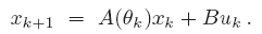
We consider linear discrete-time LPV-A systems with a parameter-varying state transition matrix and a constant input matrix

This allows one to model systems, where the system dynamics depend on scheduling signals, and this scheduling signal is measurable, but not known in advance.

An example for the computation of explicit MPC control laws for general LPV systems is shown in the LPV-MPC example. The subclass of LPV-A systems allows for simpler computations, which will be presented in the following.

The nonlinear Hénon map

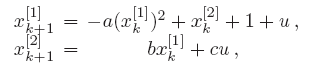
The Hénon map is a nonlinear second-order system and a popular example for chaotic systems. It is defined as

where the elements in the superscript indicate the element of the state vector. When the coefficients are \(a = 1.4\), \(b = 0.3\), the system has an unstable fix point at

In the following we will denote the fix point by \(xref\). Already small deviations from this fix point lead to chaotic behavior and the system moves along a so-called chaotic attractor:

In order to stabilize the Hénon map to the fix point, we introduce an input to obtain the controlled Hénon map

where the input coefficient is set to \(c = 0.1\).

LPV-A model of the Hénon map

If we want to compute an explicit controller with the proposed method, we have to embed the Hénon map into an LPV-A model. Due to the affine term in the Hénon map, this is not directly possible. However, the proposed algorithm easily extends to systems with affine terms in the state prediction. The Hénon map can thus be written as

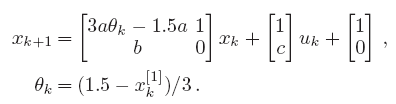
Here the scheduling parameter is an affine function of the first state and varies within [-1.5,1.5], like the state does on the chaotic attractor.

Explicit MPC for LPV-A systems

Let us find the explicit solution to a variant of the MPC problem for LPV-A systems. This will be a pretty advanced example, so let us start slowly by defining some data.

yalmip('clear')

% Model data
A1 = [ 2.1 1;0.3 0];
A2 = [-2.1 1;0.3 0];
B  = [1;0.1];
f  = [1;0];

% System sizes
nx   = 2; % Number of states
nu   = 1; % Number of inputs
ndyn = 2; % Number of vertex systems

% State and input constraints
xmin = [-10;-10];
xmax = [ 10; 10];
umin = -5;
umax =  5;

% Reference point
xref = [0.63;0.19];

% MPC data
Q   = eye(nx);
R   = 0.1;
N   = 4;
nrm = 1;

The used norm in this example is the 1-norm. To simplify the code and the notation, we create state, control and scheduling parameters in cell arrays.

% States x(k), ..., x(k+N)
x  = sdpvar(repmat(nx,1,N),repmat(1,1,N));
% Inputs u(k), ..., u(k+N) (last one not used)
u  = sdpvar(repmat(nu*ndyn,1,N),repmat(1,1,N));
% Scheduling parameter
th = binvar(repmat(ndyn,1,N),repmat(1,1,N));
% Epigraph variable
sdpvar w

Dynamic Programming Iterations

Now, instead of setting up the problem for the whole prediction horizon, we only set it up for one step, solve the problem parametrically, take one step back, and perform a standard dynamic programming value iteration.

for k = N:-1:1   % shifted: N-1:-1:0

    % Parameter simplex
    F = [uncertain(th{k}), sum(th{k}) == 1, 0 <= th{k} <= 1];
    F = [F, 0 <= w <= 10000];

    % Uncertain predictions and control
    uth = kron(th{k},eye(nu))'*u{k};    % u(th)
    Ath = [A1 A2]*kron(th{k},eye(nx));  % A(th) = A1*th1 + A2*th2 + ...   
    xp  = Ath*x{k} + f + B*uth;

    % Input constraints
    F = [F, repmat(umin,ndyn,1) <= u{k} <=  repmat(umax,ndyn,1)];

    % State constraints
    F = [F, xmin  <= x{k} <= xmax];

    % Insert step-specific code here
    % ...
    % ...

    % Solve multi-parametric problem
    [sol{k},diagnost{k},Uz{k},J{k},Optimizer{k}] = solvemp(F,obj,[],x{k},u{k});
end

In the first and the last step of the iteration, some parts of the code differ from the remaining steps. The common parts are the definition of the parameter simplex, the state update equation, the state and input constraints, the robust counterpart and the solution of the resulting multi-parametric program. In the following the step dependent code snips are listed.

First step

In the first step we rewrite the 1-norm into an epigraph formulation, and add constraints for the final state. Note that we have to manually derive the epigraph models of the sum-of-1-norms (note true any longer, example written for old version)

% |x| written as max(a[x;u]+b)
a = [-1+2*dec2decbin(0:2^nx-1,nx) zeros(2^nx,nu)];
b = zeros(2*nx,1);
% |u| written as max(c[x;u]+d)
c = [zeros(2^nu,nx) -1+2*dec2decbin(0:2^nu-1,nu)];
d = zeros(2*nu,1);

% |x|+|u| written as max(aa[x;u]+bb)
aa = repmat(a,2*nu,1) + kron(c,ones(size(a,1),1));
bb = repmat(b,2*nu,1) + kron(d,ones(size(a,1),1));

% Final state constraints
F = [F, xmin <= xp <= xmax];

% Cost function
F   = [F, aa*[Q*(xp-xref);R*uth]+bb + norm(Q*(x{k}-xref),nrm) <= w];
obj = w;

% Determine robust counterpart
[F,obj] = robustify(F,obj,[],th{k});

Intermediate steps

In the following steps we get the hyperplanes from the previous solution for the cost-to-go. We constrain the predicted states to be a feasible state for the preceding step of the DP iteration.

% Get the hyperplanes for cost-to-go
S = unique(([reshape([sol{k+1}{1}.Bi{:}]' ,nx,[])'  reshape([sol{k+1}{1}.Ci{:}]' ,[],nu)]),'rows');
a = [S(:,1:nx) zeros(size(S,1),nu)];
b = S(:,nx+1:end);

% Jp+|u| = max(a[x;u]+b)+|u|=max(a[x;u]+b)+max(c[x;u]+d)=max(aa[x;u]+bb)
aa = repmat(a,2*nu,1) + kron(c,ones(size(a,1),1));
bb = repmat(b,2*nu,1) + kron(d,ones(size(a,1),1));

% Constrain predicted state
[H,K] = value(sol{k+1}{1}.Pfinal);
F     = [F, H*xp <= K];

% Cost function
F   = [F, aa*[xp;R*uth]+bb + norm(Q*(x{k}-xref),nrm)< w];
obj = w;

% Determine robust counterpart
[F,obj] = robustify(F,obj,[],th{k});

Final step

In the last step we use the uncontrolled successor step to improve control performance. The code snip inserted into the iteration is:

% Get the hyperplanes for cost-to-go
S = unique(([reshape([sol{k+1}{1}.Bi{:}]',nx,[])' reshape([sol{k+1}{1}.Ci{:}]',[],nu)]),'rows');
a = [S(:,1:nx) zeros(size(S,1),nu)];
b = S(:,nx+1:end);

% Jp+|u| = max(a[x;u]+b)+|u|=max(a[x;u]+b)+max(c[x;u]+d)=max(aa[x;u]+bb)
aa = repmat(a,2*nu,1) + kron(c,ones(size(a,1),1));
bb = repmat(b,2*nu,1) + kron(d,ones(size(a,1),1));

% Redefine final step input
u{1} = sdpvar(nu,1); % final step input

% Input constraints
F = [umin <= u{1} <= umax];

% State update equation
xp = x{k} + f + B*u{1}; % x{1} = z

% Constrain predicted state
[H,K] = value(sol{k+1}{1}.Pfinal);
F     = [F, H*xp <= K];

% Cost function
F   = [F, aa*[xp;R*u{1}]+bb <= w];
obj = w;

Results

Finally the control performance of the Explicit LPV-MPC controller is compared to a PWA approach and the truely optimal solution for a certain scheduling parameter trajectory (for details see the above mentioned paper). Note that a robust MPC controller failed to stabilize the system.

The actual costs of the closed-loop system over a grid of initial points are depicted in the following Figure. Both the Explicit LPV-MPC controller as well as the PWA MPC controller achieve close to optimal performance (the average cost increase is 2.3 % vs. 3.9 %).

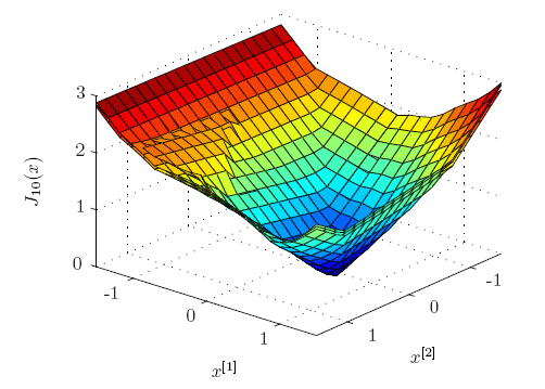
Thus both approaches seem to be reasonable ways to achieve constrained control at high sampling rates. It is worth noting that the LPV-MPC controller required 93 regions, while the PWA-MPC controller consists of 344 regions, which is a factor of more than 3 difference.