Portfolio optimization

Standard Markowitz portfolio

The standard Markowitz mean-variance portfolio problem is to select assets (relative investments \(x\)) to minimize the variance \(x^TSx\) of the portfolio profit while giving a specified expected return \(\mu^{\star}\), given historical data of mean returns \(\mu\) and covariance \(S\) of stock returns.

Let us begin by defining some random data with 10 candidate assets.

n = 10;
S = randn(n);S = S*S'/1000; % Covariance
mu  = rand(1,n)/100;        % Expected return       

We introduce a vector x to model the position in each asset, and solve the standard Markowitz portfolio problem (no short positions) and aim for an expected return equal to the average historical return of all assets.

x = sdpvar(n,1);
mutarget = mean(mu);
F = [sum(x) == 1, x>=0, mu*x == mutarget];
optimize(F,x'*S*x)
value(x)

An alternative approach is to limit the variance, and maximize the expected return. Let us maximize the return while constraining the variance to be less than the variance for a portfolio with equal positions in all assets (this model leads to a quadratically constrained problem, hence you need a QCQP or SOCP capable solver such as sedumi, sdpt3, GUROBI, MOSEK, or CPLEX)

F = [sum(x) == 1, x>=0];
F = F + [x'*S*x <= sum(sum(S))/n^2];
optimize(F,-mu*x)
value(w)

Yet another proposal is to maximize the Sharpe ratio \(\frac{x^T(\mu-\mu_0)}{\sqrt{x^TSx}}\) where \(\mu_0\) is the return of a risk-free asset, i.e., the excess return per unit standard deviation. A first sight, this is terribly nonlinear and can indeed also be non-convex. However, it can easily be converted to a quadratic program. In principle, we note that the normalization that the weights should sum to 1 is rather arbitrary, we just want it to be non-zero and the important result is the relative sizes. We can just as well use a new set of weights \(z\) with the constraint that \(z^T(\mu-\mu_0)=1\). With this, our objective is maximization of \(\frac{1}{\sqrt{z^TSz}}\), i.e., minimization of \(z^TSz\)

mu0 = 0.001;
z = sdpvar(n,1);
optimize([z'*(mu(:)-mu0)==1, z>=0],z'*S*z)
x = value(z)/sum(value(z))

The solutions to the problems above typically leads to a portfolio with shares in most assets. This is typically not wanted, since it leads to increased transaction and administration costs.

Cardinality & structurally constrained portfolios

An alternative is to only allow a limited number of non-zero positions. This is easily modeled using the nnz operator, and leads to a mixed integer quadratic programming problem. Let us limit the number of positions to 4 (since nnz requires a MILP model, we explicitly upper bound the variable x to help the big-M reformulation). Please note that cardinality constrained portfolio selection yields extremely hard problems.

mutarget = mean(mu);
F = [sum(x) == 1, 1>=x>=0, mu*x == mutarget];
F = F + [nnz(x) <= 4];
optimize(F,x'*S*x)
value(x)

To ensure a balanced portfolio, constraints on smallest and largest fraction could be useful. We can do this by hand using the following model, where we aim for a portfolio where no asset accounts for more than 80%, but at the same time no non-zero positions are smaller than 10%.

d = binvar(n,1);           % models if variable is nonzero
F = [sum(x) == 1, 1>=x>=0, mu*x == mutarget];
F = F + [sum(d) <= 4]   % At most 4 positions
F = F + [x <= d];       % If d(i)==0 then x(i) = 0
F = F + [x >= 0.1*d];   % If d(i)==1 then x(i) >= 0.1
F = F + [x <= 0.8];     % No position >= 0.8
optimize(F,x'*S*x)
value(w)

An equivalent model can be obtained by using the command semivar. The drawback with the following code is that it can be slightly less efficient since it introduce separate binary variables for the cardinality constraint and the semi-continuous position vector. An efficient pre-solve in the integer solver should be able to detect these redundant variables though.

w = semivar(n,1);      % Either 0...
F = [0.1 <= x <= 0.8]; % ...or between bounds
F = [F, sum(x) == 1, mu*x == mutarget];
F = [F, nnz(x) <= 4];      % At most 4 positions
optimize(F,x'*S*x)
value(w)

The following portfolio only allows fixed sizes of the positions, while aiming for the target return

w = sdpvar(n,1);
F = [sum(x) == 1, 1>=x>=0];
F = [F, ismember(x,0:0.1:1)];  % Sizes in steps of 10%
optimize(F,x'*S*x + (mu*x - mutarget)^2)
value(w)

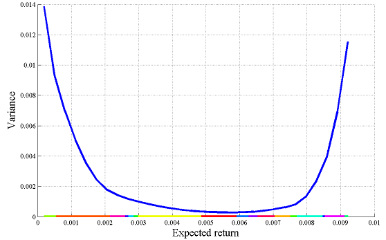
The efficient frontier

A school-book example of parametric optimization is the efficient frontier in the Markowitz portfolio. This is the lowest possible variance \(x^TSx\) achievable, when striving for a particular profit.

Repeated solutions using the optimizer command

Solving many problems with only a small change in the setup can in some cases be done efficiently using the optimizer command. This command allows us to create an object which takes the target return as input, and returns the variance and portfolio assignments as outputs. By using the optimizer command instead of explicitly setting up a new problem and calling optimize, the overhead can be reduced drastically.

x = sdpvar(n,1);
sdpvar mutarget
F = [sum(x) == 1, x>=0, mu*x == mutarget];
Portfolio = optimizer(F,x'*S*x,sdpsettings('verbose',0),mutarget,[x'*S*x;x]);

Optimal portfolios can now easily be computed in one shot.

targets = linspace(min(mu),max(mu),100);
solutions = Portfolio{targets};
plot(targets,solutions(1,:))

Multiparametric approach

We can alternatively compute and plot this curve, if MPT is installed.

x = sdpvar(n,1);
sdpvar mutarget
F = [sum(x) == 1, x>=0, mu*x == mutarget];
[sol,dgn,aux,Valuefcn,xoptimal] = solvemp(F,x'*S*x,[],mutarget);
plot(Valuefcn);

The minimum risk portfolio and the associated variance at the target profit that we computed in the beginning of this example can be extracted from the parametric solution

assign(mutarget,mean(mu))
value(xoptimal)
value(Valuefcn)