Simulink models with YALMIP components
All files and models in this article are available in yalmipsimulink.zip
To begin with, some parts of a Simulink model are compiled for performance, and this compiler does not support code which involves object oriented code. Hence, it fails when it encounters any kind of YALMIP related code. In practice, this means that all YALMIP code has to be placed in a so called Interpreted MATLAB function. This implies that you cannot compile Simulink with YALMIP to a target (such as a DSP or something similar). At least, I have not come up with any way to do this.
Second, since Simulink typically is used for simulations, the YALMIP code will most likely be called a large number of times. Hence, it is important to create efficient YALMIP code, minimizing overhead and unnecessary computations by using an optimizer object. In many cases this is possible, but sometimes it is hard and you simply have to accept that the simulations run slowly if you want to use highl-level YALMIP code.
To illustrate YALMIP and Simulink, we will implement an MPC controller using a couple of different strategies.
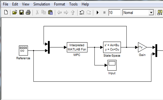
As a start, we create a basic Simulink model with a linear state-space model and an Interpreted MATLAB function which will hold the code to call the MPC controller.
We also create a file setupsimulation.m which sets up the data for the model (already included in the yalmipsimulink.zip)
% System
Plant = ss(tf(1,[1 0 0]));
A = Plant.A;
B = Plant.B;
C = Plant.C;
D = Plant.D;
% Global sampling-time
Ts = 0.1;
% Initial state for simulation
x0 = [1;1];
As simple (and slow) as possible
Our first try (MPCSimulationSlowest.mdl) will be a naive approach where we simply place all MPC code in a file, and run this file every time a new state comes in (based on the sample-time Ts). Everything will be defined from scratch, so the code will naturally run very slowly. Hence, we create a file called SlowestMPCController.m which takes a two inputs, the state and the reference, and returns the scalar control signal. Note the lazy coding here, we define and compute everything every time the function is called. Simple but slow.
function uout = SlowestMPCController(currentx,r)

% Compute discrete-time dynamics
Plant = ss(tf(1,[1 0 0]));
A = Plant.A;
B = Plant.B;
C = Plant.C;
D = Plant.D;
[nx,nu] = size(B);
Ts = 0.1;
Gd = c2d(Plant,Ts);
Ad = Gd.A;
Bd = Gd.B;

% Define data for MPC controller
N = 10;
Q = 10;
R = 0.1;

% Avoid explosion of internally defined variables in YALMIP
yalmip('clear')

% Setup the optimization problem
u = sdpvar(repmat(nu,1,N),repmat(1,1,N));
x = sdpvar(repmat(nx,1,N+1),repmat(1,1,N+1));

% Define simple standard MPC controller
% Current state is known so we replace this
x{1} = currentx;
constraints = [];
objective = 0;
for k = 1:N
    objective = objective + (r-C*x{k})'*Q*(r-C*x{k})+u{k}'*R*u{k};
    constraints = [constraints, x{k+1} == Ad*x{k}+Bd*u{k}];
    constraints = [constraints, -5 <= u{k}<= 5];
end

% Solve!
sol = optimize(constraints,objective);

if sol.problem
 % Debug, analyze, fix!
else
 % ...and return the optimal input
 uout = value(u{1});
end
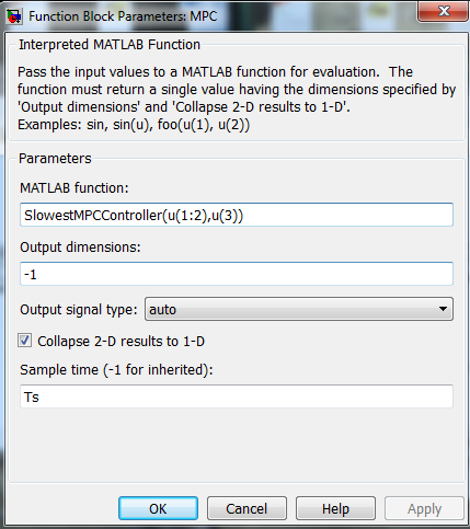
The MPC block is setup to call the function. Note the sample-time, which should be consistent with the sample-time used in the definition of the MPC controller. The state and the reference signals have been Muxed in the Simulink model, so we now extract the suitable elements in accordance with our function definition.
and we are ready to run
setupsimulation
tic;sim('MPCSimulationSlowest');toc
Elapsed time is 62.086316 seconds.
Awfully slow as promised. Simulating 10 seconds takes over a minute! Not too surprising though, since every call to the controller takes close to a second, despite using a fast QP solver (the computations here were performed using GUROBI).
tic
SlowMPCController(x0,1);
toc
Elapsed time is 0.719190 seconds.
At this point, we could start working with global variables, or sending predefined data to the function. For instance, it is of course silly to discretize the system every call. However, the major problem is most likely the redefinition of decision variables and constraints, and calling optimize which involves a lot of high-level code to analyze and compile the model to a numerical format.
Slightly less simple and slightly faster
Our first improvement will be to avoid redefinition of everything every sample. The approach here uses persistent variables (variables which aren’t cleared during repeated calls) and a YALMIP model where the initial state and the reference are defined as sdpvar objects, and then constraining these when we want the solution for a particular state and reference. The Simulink model is available in MPCSimulationSlow.mdl and the controller is defined in SlowMPCController.m. Note that we have have added a clock to the model, which is sent to the controller object. If the time is 0, the model is setup, otherwise, the persistingly available model is used.
function uout = SlowMPCController(currentx,currentr,t)

persistent constraints
persistent objective
persistent x u r
persistent ops

if t == 0
    % Compute discrete-time dynamics
    Plant = ss(tf(1,[1 0 0]));
    A = Plant.A;
    B = Plant.B;
    C = Plant.C;
    D = Plant.D;
    [nx,nu] = size(B);
    Ts = 0.1;
    Gd = c2d(Plant,Ts);
    Ad = Gd.A;
    Bd = Gd.B;

    % Define data for MPC controller
    N = 10;
    Q = 10;
    R = 0.1;

    % Avoid explosion of internally defined variables in YALMIP
    % Not really necessary as we only define the model once, but anyhow...
    yalmip('clear')

    % Setup the optimization problem
    u = sdpvar(repmat(nu,1,N),repmat(1,1,N));
    x = sdpvar(repmat(nx,1,N+1),repmat(1,1,N+1));
    sdpvar r
    % Define simple standard MPC controller
    % Current state is known so we replace this
    constraints = [];
    objective = 0;
    for k = 1:N
        objective = objective + (r-C*x{k})'*Q*(r-C*x{k})+u{k}'*R*u{k};
        constraints = [constraints, x{k+1} == Ad*x{k}+Bd*u{k}];
        constraints = [constraints, -5 <= u{k}<= 5];
    end

    % Solve, and constrain the symbolic initial state and reference
    % Don't hide solver logs when developing the controller
    % Log is not shown in command window, you either have to use a break
    % and run line manually, or look in debug window
    % Once everything works, you can turn off display
    ops = sdpsettings('verbose',1);
    sol = optimize([constraints,x{1} == currentx, r == currentr],objective,ops);
    if sol.problem
       % Debug, analyze, fix
    else
       uout = value(u{1});
     end
else
    % Solve, and constrain the symbolic initial state and reference
    % Don't hide solver logs when developing the controller
    % Log is not shown in command window, you either have to use a break
    % and run line manually, or look in debug window
    % Once everything works, you can turn off display
    sol = optimize([constraints,x{1} == currentx, r == currentr],objective,ops);
    if sol.problem
       % Debug, analyze, fix
    else
       % ...and return the optimal input
       uout = value(u{1});
    end
end
The calls to the controller are now roughly twice as fast once the model has been setup at t=0, but the simulation is still slow enough to almost warrant a coffee break.
>> tic;SlowMPCController(x0,1,0);toc %Includes setup at t=0
Elapsed time is 0.587677 seconds.
>> tic;SlowMPCController(x0,1,0.1);toc %No setup for t>0
Elapsed time is 0.255265 seconds.

>> setupsimulation
tic;sim('MPCSimulationSlow');toc
Elapsed time is 25.754945 seconds.
However, significant overhead still remains, as optimize is called every iteration, requiring a lot of back-end code (modeling of operators, convexity analysis, choice of solver, compilation of numerical data etc etc). To avoid this, we implement the controller using an optimizer object.
As fast as it gets
Changing the slow MPC controller code to a version using an optimizer is trivial. The models are implemented in MPCSimulation.mdl and MPCController.m. Note that the only persistent variable now is the controller object, nothing else is required.
Best practice: Never use an optimizer approach before you know everything works as expected, and when debugging crank up verbosity level (to see solver logs when using optimizer you have to set the level to 2) and to see displayed outputs when running in Simulink you have to put a break in the code and manually run the line.
function uout = MPCController(currentx,currentr,t)

persistent Controller

if t == 0
    % Compute discrete-time dynamics
    Plant = ss(tf(1,[1 0 0]));
    A = Plant.A;
    B = Plant.B;
    C = Plant.C;
    D = Plant.D;
    [nx,nu] = size(B);
    Ts = 0.1;
    Gd = c2d(Plant,Ts);
    Ad = Gd.A;
    Bd = Gd.B;

    % Define data for MPC controller
    N = 10;
    Q = 10;
    R = 0.1;

    % Avoid explosion of internally defined variables in YALMIP
    yalmip('clear')

    % Setup the optimization problem
    u = sdpvar(repmat(nu,1,N),repmat(1,1,N));
    x = sdpvar(repmat(nx,1,N+1),repmat(1,1,N+1));
    sdpvar r
    % Define simple standard MPC controller
    % Current state is known so we replace this
    constraints = [];
    objective = 0;
    for k = 1:N
        objective = objective + (r-C*x{k})'*Q*(r-C*x{k})+u{k}'*R*u{k};
        constraints = [constraints, x{k+1} == Ad*x{k}+Bd*u{k}];
        constraints = [constraints, -5 <= u{k}<= 5];
    end

    % Define an optimizer object which solves the problem for a particular
    % initial state and reference
    % Don't hide solver logs when developing the controller
    % Log is not shown in command window, you either have to use a break
    % and run line manually, or look in debug window
    % Once everything works, you can allow optimizer to turn off display
    ops = sdpsettings('verbose',2);
    Controller = optimizer(constraints,objective,[],{x{1},r},u{1});

    % And use it here too
    [uout,problem] = Controller(currentx,currentr);
    if problem
       % You have to sort out what to do when solve fails!
    end

else
    % Almost no overhead
    [uout,problem] = Controller(currentx,currentr);
    if problem
       % You have to sort out what to do when solve fails!
    end
end
Calling the controller the first time will still take time since it must set up the whole optimization model, but for all other samples, the overhead is drastically reduced and the whole simulation is completed in a couple of seconds.
>> tic;MPCController(x0,1,0);toc
Elapsed time is 0.666965 seconds.
>> tic;MPCController(x0,1,0.1);toc
Elapsed time is 0.008276 seconds.

>> setupsimulation
>> tic;sim('MPCSimulation');toc
Elapsed time is 2.075632 seconds.
