Unit commitment
Complete code, click to expand!
A classical problem in scheduling and integer programming is the unit commitment problem. In this problem, our task is to turn on and off power generating plants, in order to meet a forecasted future power demand, while minimizing our costs. We have several different power plants with different characteristics and running costs, and various constraints on how they can be used. We will start with a very simple model, and then expand this model with more advanced features. To make the code easy to read, we will write it in a verbose non-vectorized format.
Tip: The most important thing we learn in this example is that you never multiply binary variables with continuous variables to model on/off behavior. Instead, we derive equivalent linear presentations.
Note that this is a completely fictitious example created by someone (me) with very little exposure and experience from this field. The purpose is to highlight modeling tricks and YALMIP, not to give a tutorial or best-practice description on unit commitment problems.
Before running these examples, you must install a strong MILP solver (if you don’t have one installed, YALMIP will use its very naive internal integer solver BNB which will fail to solve most problems here in reasonable time, if at all).
Data for the model
To begin with, we assume we have \(N=3\) power generating plants of different types (nuclear, hydro, gas, oil, coal, …). Each of these plants have a maximum power capacity, and a minimum capacity when turned on. Our scheduling problem is solved over 48 time units (hours,days,…), and the forecasted power demand is given by a periodic function. The cost of running plant \(i\) for one time unit is given by a quadratic function \(Q_{ii} P_i^2 + C_i P_i\) where \(P_i\) is the delivered power from plant \(P_i\).
Nunits = 3;
Horizon = 48;

Pmax = [100;50;25];
Pmin = [20;40;1];

Q = diag([.04 .01 .02]);
C = [10 20 20];

Pforecast = 100 + 50*sin((1:Horizon)*2*pi/24);
A first model with linear on-off modelling
The model will be composed of two variables. The first is a binary variable which controls if unit \(i\) is turned on at time \(k\), and the second variable is a continuous variable representing the power delivered by plant \(i\) at time \(k\).
onoff = binvar(Nunits,Horizon,'full');
P     = sdpvar(Nunits,Horizon,'full');
A typical mistake made now when modeling these things, is to start multiplying the onoff variables with the power variables P, following the logic that the power from a plant is given by the product of onoff and P. This is an extremly bad way to model these things, since they will move us outside the comfortable world of mixed integer linear and quadratic programming. Instead, the multiplication should be done implicitly through logic constraints. If onoff is 0, P should be zero, and if onoff is 1, P should be allowed to be between its lower and upper bounds. This can be implemented using the command implies, but we will model it manually here.
We start building our model based on this logic (remember, this can be vectorized, we use for-loops only to make the model easier to understand)
Constraints = [];
for k = 1:Horizon
  Constraints = [Constraints, onoff(:,k).*Pmin <= P(:,k) <= onoff(:,k).*Pmax];
end
The total demand delivered at each time instant must be sufficiently large
for k = 1:Horizon
  Constraints = [Constraints, sum(P(:,k)) >= Pforecast(k)];
end
The total running cost over the forecasted horizon is computed
Objective = 0;
for k = 1:Horizon
  Objective = Objective + P(:,k)'*Q*P(:,k) + C*P(:,k);
end
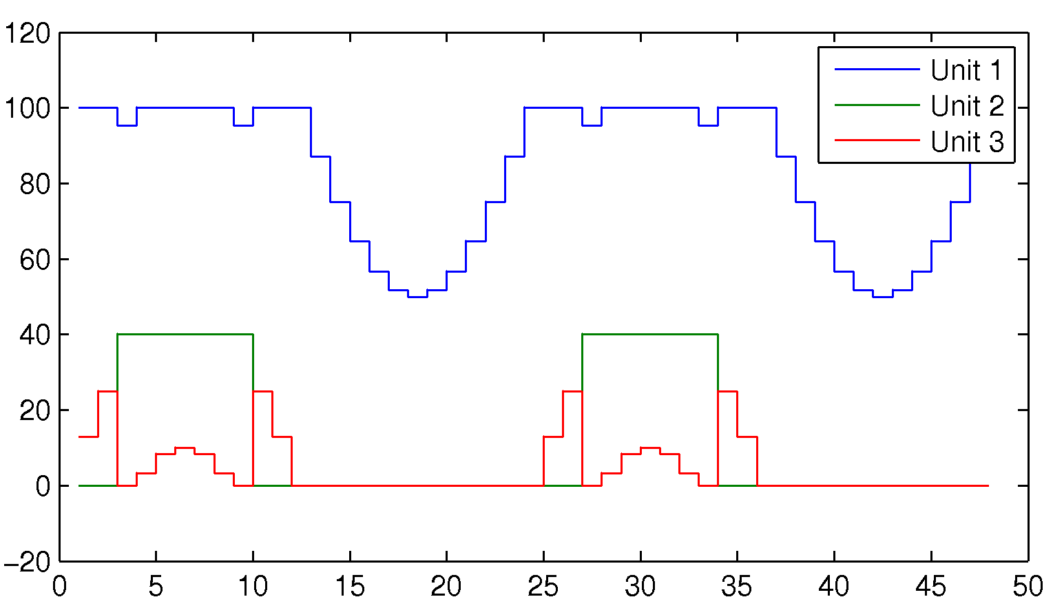
The first simple model is complete, and we can solve the problem and display the results (this requires that you have an efficient mixed-integer QP solver installed.)
Tip: Always turn on full display and debug mode when developing new models. Once you are certain everything works as expected, you can turn off display for improved performance.
ops = sdpsettings('verbose',1,'debug',1);
optimize(Constraints,Objective,ops)
stairs(value(P)');
legend('Unit 1','Unit 2','Unit 3');
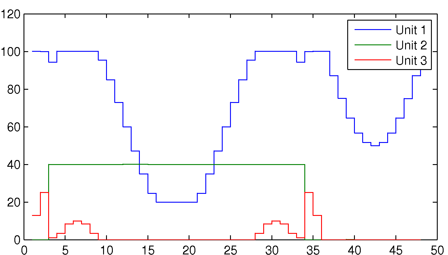
Adding minimum up- and down-time
The model above is far from realistic, and one of the main flaws is that it assumes that we can turn on and off the plants arbitrarily. Most often, if a plant is turned on, it has to run for a number of time units, and when turned off, it will be gone for a number of time units (restarting is complicated etc). We define two new variables describing these plant characteristics
minup   = [6;30;1];
mindown = [3;6;3];
Hence, when plant 1 is turned on, it has to be on for at least 6 consecutive time units, and when plant 2 is switched off, it will remain off for 6 time units.
Let us now describe these properties through linear constraints involving binary variables, and we begin with the minimum up-time constraint. If plant i is switched on, it has to remain on for minup(i) time units. This can be stated as: if plant is off at time k-1 and on at k, then it is must be on at time k+1, k+2,…,k+minup(i)-1. The trick now is to get an indicator for being switched on. Convince your self that onoff(k)-onoff(k-1) is 1 when this happens, otherwise it is 0 or -1. Hence, the following model will work
for k = 2:Horizon
 for unit = 1:Nunits
  % indicator will be 1 only when switched on
  indicator = onoff(unit,k)-onoff(unit,k-1);
  range = k:min(Horizon,k+minup(unit)-1);
  % Constraints will be redundant unless indicator = 1
  Constraints = [Constraints, onoff(unit,range) >= indicator];
 end
end
The down-time constraint is created in a similar fashion.
for k = 2:Horizon
 for unit = 1:Nunits
  % indicator will be 1 only when switched off
  indicator = onoff(unit,k-1)-onoff(unit,k);
  range = k:min(Horizon,k+mindown(unit)-1);
  % Constraints will be redundant unless indicator = 1
  Constraints = [Constraints, onoff(unit,range) <= 1-indicator];
 end
end
ops = sdpsettings('verbose',2,'debug',1);
optimize(Constraints,Objective,ops);
stairs(value(P)');
legend('Unit 1','Unit 2','Unit 3');
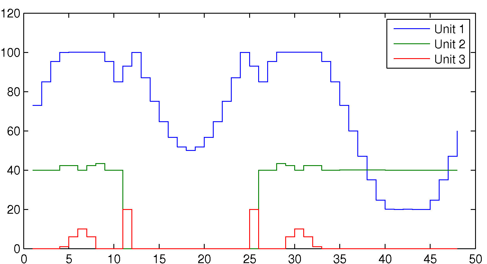
Quantized power-levels
Some plants can only be run in a finite number of configurations, thus making the delivered power a quantized variable. Here, we assume plant 3 is limited in such a way and the quantization is modelled using the ismember operator.
Unit3Levels = [0 1 6 10 12 20];
for k = 1:Horizon
  Constraints = [Constraints, ismember(P(3,k),Unit3Levels)];
end
optimize(Constraints,Objective);
stairs(value(P)');
legend('Unit 1','Unit 2','Unit 3');
Efficient simulation
As a finale, let us simulate this plant control strategy in closed-loop. To do this we have to make some changes. To begin with, we must introduce a history. The action we take now depends on our past. If we turned on plant two 10 time units ago, we must still have it on, etc. The second thing we should do is to make the simulation efficient, by avoiding a complete redefinition of the whole optimization problem every time instant. To do so, we use the optimizer command. Finally, to make it realistic, we should have some disturbances on the power demand, and to cope with this, we add a simple slack on the power demand constraint, and penalize this slack in the objective function.
In order to use the optimizer command, parameters that change in each iteration must be declared as sdpvar objects. Things that change are the forecasts and the sliding history. As before, we use a forecast of 48 time units, and to cope with the up- and down-time constraints, we need a history of at least 30 time units.
Nhist = max([minup;mindown]);
Pforecast = sdpvar(1,Horizon);
HistoryOnOff = sdpvar(Nunits,Nhist,'full');
DemandSlack = sdpvar(1,Horizon);
PreviusP = sdpvar(3,1);
DemandPenalty = 1000;
ChangePenalty = 1000;
Setup the basic part of the model
Constraints = [];
Objective = 0;
for k = 1:Horizon
  Constraints = [Constraints, onoff(:,k).*Pmin <= P(:,k) <= onoff(:,k).*Pmax];
  Constraints = [Constraints, sum(P(:,k))+DemandSlack(k) >= Pforecast(k)];
  Constraints = [Constraints, DemandSlack(k) >= 0];
  Objective = Objective + P(:,k)'*Q*P(:,k) + C*P(:,k);
  Objective = Objective + DemandPenalty*DemandSlack(k);
end
To simplify the code, we create a separate general function to define up-time constraints.
function C = consequtiveON(x,minup)
if min(size(x))==1
    x = x(:)';
end
if size(x,1) ~= size(minup,1)
    error('MINUP should have as many rows as X');
end
Horizon = size(x,2);
C = [];
for k = 2:size(x,2)
    for unit = 1:size(x,1)
        % indicator will be 1 only when switched on
        indicator = x(unit,k)-x(unit,k-1);
        range = k:min(Horizon,k+minup(unit)-1);
        % Constraints will be redundant unless indicator = 1
        affected = x(unit,range);
        if strcmp(class(affected),'sdpvar')
        % ISA behaves buggy, hence we use class+strcmp
            C = [C, affected >= indicator];
        end
    end
end
This function is now used on our concatenated history and future sequences. Note that a down-time constraint can be formulated by applying a suitably defined up-time constraint
Constraints = [Constraints, consequtiveON([HistoryOnOff onoff],minup)];
Constraints = [Constraints, consequtiveON(1-[HistoryOnOff onoff],mindown)];
We add a term to the objective function to penalize changes in the control.
for k = 2:Horizon
   Objective = Objective + ChangePenalty*norm(P(:,k)-P(:,k-1),1);
end
Objective = Objective + ChangePenalty*norm(P(:,1)-PreviusP,1);
We are now ready to create our optimizer object. Our optimizer object solves the optimization problem for a particular instance of the forecast demand and history, and returns the optimal powers and on-off sequences. We’re still running with full diagnostic display to be able to detect any issues you might have with your installation.
Parameters = {HistoryOnOff, Pforecast, PreviusP};
Outputs = {P,onoff};
ops = sdpsettings('verbose',2,'debug',1);
Controller = optimizer(Constraints,Objective,ops,Parameters,Outputs);
We create a history where we assume plant one has been running at 100, plant two at 40, and the third plant has been turned off.
oldOnOff = repmat([1;1;0],1,Nhist);
oldP = repmat([100;40;0],1,Nhist);
Simulate!
for k = 1:500
% Base-line forecast
forecast = 100;
% Daily fluctuation
forecast = forecast + 50*sin((k:k+Horizon-1)*2*pi/24);
% Some other effect
forecast = forecast + 20*sin((k:k+Horizon-1)*2*pi/24/7);
% and yet some other effect
forecast = forecast + randn(1,Horizon)*5;
[solution,problem] = Controller{oldOnOff, forecast, oldP(:,end)};
optimalP = solution{1};
optimalOnOff = solution{2};
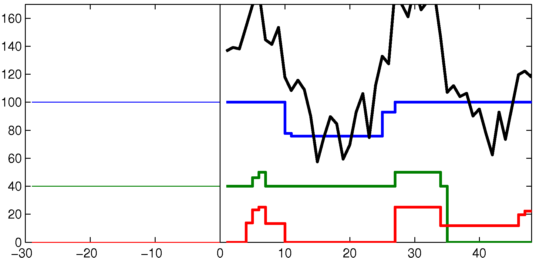
hold off
stairs([-Nhist+1:0 1:Horizon],[oldP optimalP]');
hold on
stairs(1:Horizon,forecast,'k+');
axis([-Nhist Horizon 0 170]);
drawnow
pause(0.05);
% Shift history
oldP = [oldP(:,2:end) optimalP(:,1)];
oldOnOff = [oldOnOff(:,2:end) optimalOnOff(:,1)];
end
Play around with the various prices and characteristics, and you will see that you can create very different simulations.
If your browser supports animated png, you will see an animation of the simulation in the figure below.