Sorting with linear programming, or?

This example currently only runs on the develop branch

A discussion on stackexchange led to some experiments and an interesting case where a linear programming formulation is absolutely horrible compared to an approach where a general nonlinear solver used. We thus have a problem where the standard rule that we should solve problems as a linear programs if possible is violated.

So can it be more efficient to solve a linear program using a nonlinear solver than a dedicated LP solver? Depends on what you mean with a linear program.

The problem

The problem discussed which triggered this example is

The norm in the objective and the norm in the constraints are trivially LP-representable and do not pose any problems, neither in theory nor practice. The problem is the first term which involves a sorting operator. Note that it does not explicitly require the sorted vector, it only asks for the inner products of the sorted vector and a given vector \(p\). In our discussion here, we assume sort is in descending order.

For arbitrary \(p\) this is not a convex problem. This can easily be seen if we consider the case where all but the last elements in \(p\) are 0, and the last element is 1. The inner product then simply returns the smallest element of the vector, and we know that \( \min \) is a concave function, hence the problem is non-convex as we are minimizing the objective.

MILP sorting

Sorting a vector is in general is a very complex operation to describe in an optimization model. Assuming a descending sort, we can describe a sorted vector \(s = \text{sort}(x)\) via the constraints \(s = Px, s_i \geq s_{i+1} \) where \(P\) is a binary permutation matrix, \( \sum_i P_{ij} = 1, \sum_j P_{ij}=1\). To arrive at a MILP representation, a linearization (i.e. big-M representation) of the product \(Px\) is needed. Hence, the full model will not only introduce the large binary matrix \(P\) but also a large amount of additonal variables and constraints to implement the linearization. This is the model you obtain if you use the command sort in YALMIP.

In the general case, the problem is non-convex and we have no hope of an LP representation so we start our experiments with the MILP formulation on a small random case.

n = 4;
m = 10;
p = randn(m,1);
R = randn(m,n);
w0 = randn(n,1);

w = sdpvar(n,1);
objective = sort(R*w,'descend')'*p+norm(w-w0,1);
Model = [norm(w,inf)<=1];    
optimize(Model,objective);

Increasing the problem size will quickly lead to problems where the solution-time starts to become problematic. In this general case there is not much to do (unless you are clever enough to come up with a better model than the one YALMIP uses, or you use a nonlinear solver as we do below, and accept that you solve a nonlinear non-smooth non-convex problem…)

LP to the rescue (?)

The problem here does not require the sorted vector explicitly, but only needs the result from the inner product \( \text{sort}(Rw)^Tp\) for a non-negative non-increasing vector \( p\). With the sorted vector having length \(m\), this can alternatively be stated as the weighted ordered sum of m largest elements of the vector, i.e., the limiting case of the operator weighted ordered sum of k largest elements which not only is convex but also linear-programming representable.

Hence, all we have to do is to replace the call to sort and the inner product with a call to sumk, and we have converted the model to an LP (after making sure we have a convex problem by generating a \(p\) satisfying the assumptions).

p = rand(m,1);p = sort(p,'descending');

objective = sumk(R*w,m,p)+norm(w-w0,1);
Model = [norm(w,inf)<=1];    
sol = optimize(Model,objective);

Promising and easily solved, and when we start increasing the problem size, it quickly becomes much faster than the MILP approach, which is to be expected. However, for rather modest problem sizes, also this model starts to run into performance issues.

The problem here is that an LP representation of the sum of the k largest elements grows quickly when k is large. Our original problem has \(n\) variables, and to represent the two norms, this grows to \(2n+1\) variables with an additional introduction of \(4n\) constraints. This is no big deal and is a fairly modest increase. The weighted ordered sum of k largest elements on the other hand introduces \(m k + k\) new variables and \(2mk\) constraints. Since we have \(k=m\) this means we have quadratic growth in the size of the sorted vector. Already for a modest case where the length of the sorted vector is 1000 we are working with an LP with millions of variables and constraints. The LP-representability comes at an enormous price here. We all fear exponential growth, but already quadratic growth can be a devastating slap in the face.

NLP - doing the forbidden

We have all learned to model things in a problem class which is as simple as possible. We celebrated above when we managed to derive an LP, but is it really sensible here? We have a convex problem in \(n\) variables, but to solve this using an LP we work with an intermediate expression of size \(m\) (in this application larger than \(n\) which requires \(O(m^2)\) variables and constraints to be modelled.

Instead, let us take a completely different approach where we stay in the original variables (except those variables required to represent the norms). We can just as well see this as a general nonlinear program and solve it using our favorite nonlinear solver. If the problem is convex, the solver should perform well.

Some operators in YALMIP are modelled differently depending on which solver is used. If you use exp and a general nonlinear solver, the operator is working just as you would expect, YALMIP returns the function value and gradient to any solver asking for it. If you on the other hand use an exponential cone capable solver, it is modelled in a completely different conic way. In a similiar fashion, some operators are modelled differently depending on whether they can be represented using convex LP representations, or if the situation calls for an MILP representation. The sort operator and the sumk does not support anything but the MILP and LP representation respectively though, so we cannot use these with a nonlinear solver while staying in the original space

One way to proceed is to implement a new operator in YALMIP which computes the function value and gradient. This is easy to do, but more conveniently we use a method where we define the operator via the blackbox command.

We start with a setup which only returns the function values to the solver. This means we have to use a solver which is capable of performing numerical differentiation. To avoid creating any file at all we use an anonymous function. Any nonlinear solver will work, but here we specify FMINCON with its active-set algorithm.

f = @(w)(sort(R*w,'descend')'*p);
objective = blackbox(f,w)+norm(w-w0,1);

ops = sdpsettings('solver','fmincon','fmincon.algorithm','active-set');
optimize(Model,objective,ops)

If you test this and compare with solutions from the LP and MILP approach, you will find that the nonlinear solver indeed finds the optimal solution. Most impressively though, it is several orders of magnitude faster than the LP model on larger models. For a model of size \(n=100, m=1000\) the nonlinear model is solved in a few seconds while the LP model requires close to an hour and completely bogs down a standard computer due to excessive memory demand.

Numerical differentiation works well here, but we can supply a derivative too if we want to be fancy. The expression we work with is not differentiable as it is piecewise affine, so we must trust that our nonlinear solver is able to cope with this. If the vector happened to be sorted, the derivative would be \(R^Tp\). However, the sort operation must be taken into account, and it turns out that the gradient (or sub-gradient to be more precise) can be computed with

function df = myderivative(w,R,p)
[~,order] = sort(R*w,'descend');
df = R(order,:)'*p;

With this file available, we can run the code again, but this time with a supplied gradient.

f  = @(w)(sort(R*w,'descend')'*p);
df = @(w)myderivative(w,R,p);
objective = blackbox(f,w,df)+norm(w-w0,1);

optimize(Model,objective,ops)

The difference is minor, but it is nice to know that we are giving the nonlinear solver all the information we can.

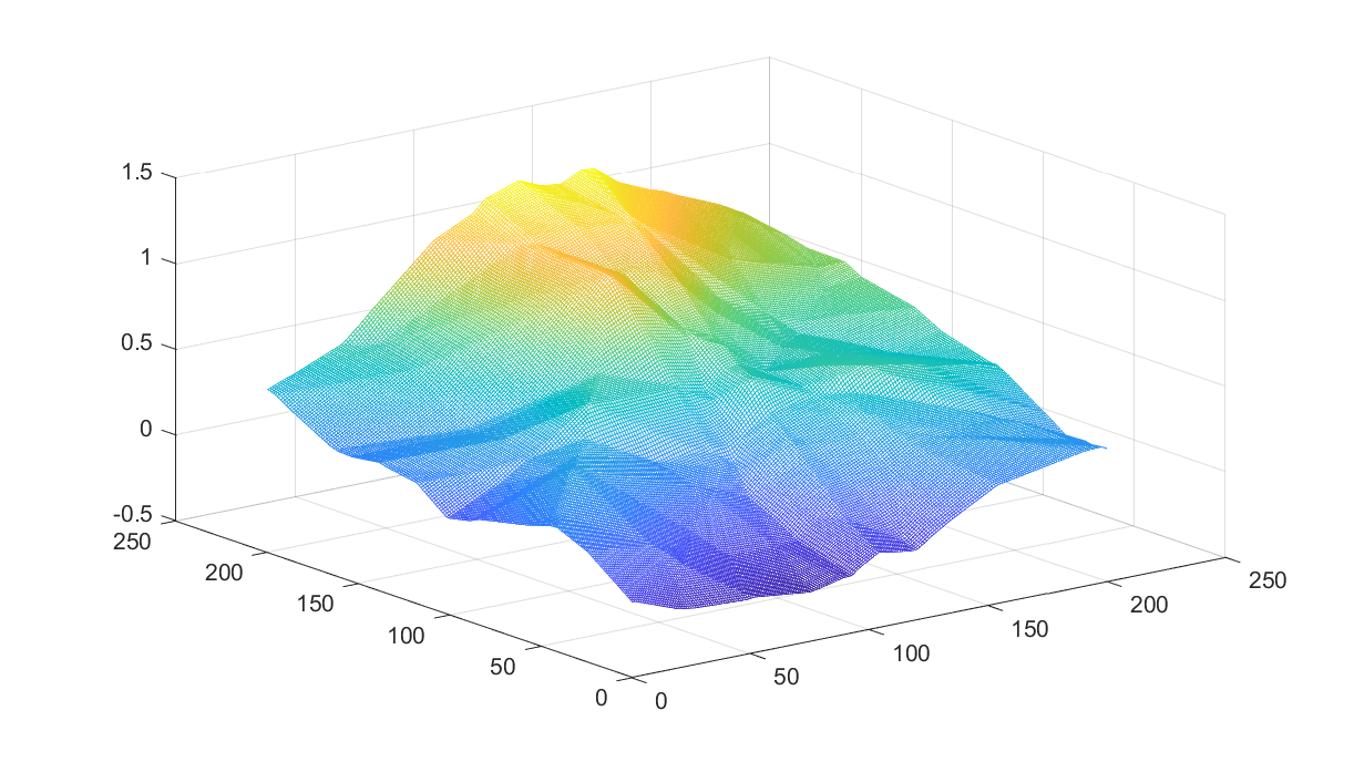
Looking at the function

Just for fun, let us illustrate what the function looks like, by plotting a random projection from a random 4-dimensional case

p = sort(rand(10,1),'descend');
R = randn(10,4);
z = rand(1,2);
x = -1:0.01:1;
y = -1:0.01:1;
for i = 1:length(x)
    for j = 1:length(y)
        w = [x(i);y(j);z];
        s = sort(R*w,'descend');
        J(i,j) = sum(s'*p);
    end
end
mesh(x,y,J)

The facet structure is visible sometimes (remember, the function is LP-representable thus guaranteed to be piecewise affine).

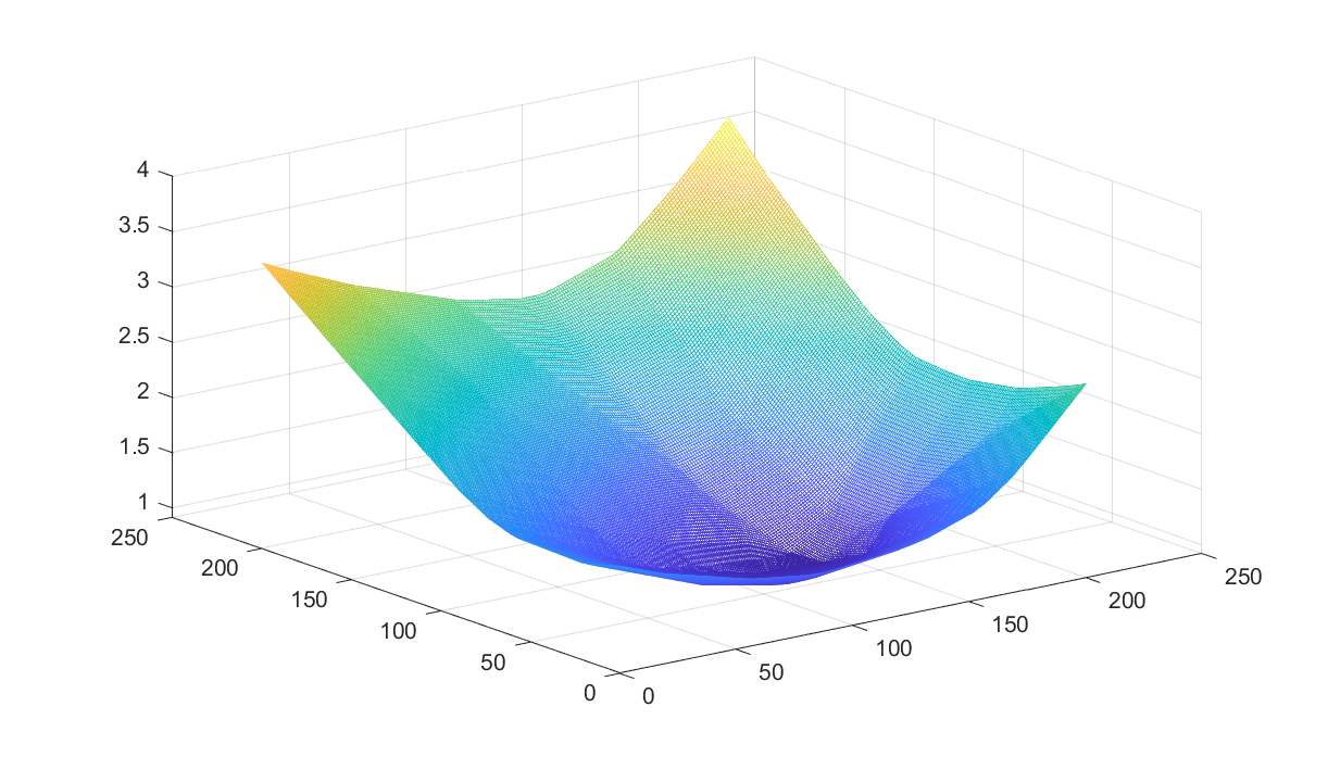
If you remove the sorting from the generation of \(p\) you will see that convexity no longer is guaranteed (it is still piecewise afffine though, as we can represent it using a MILP).