Extensions on the optimizer

The optimizer has been revamped significantly internally, and comes with new features and simplified use.

For those of you who have missed this feature, optimizer allows you to define a parameterized optimization problem which YALMIP precompiles to its internal numerical format. This object can then be instantiated for particular values on the parameters. This allows for, e.g., rapid simulation and experimentation with optimization problems, as most of the YALMIP overhead is removed from the loop.

Consider the problem of investigating the optimal value \(x\) in the optimization problem \(\textbf{min}_x~ (x-b)^2~\textbf{subject to}~ -a\leq x \leq a\), as \(a\) and \(b\) varies. Creating an optimizer object for this setup is essentially done in the same fashion as when we solve the optimization problem, except that we declare parameters (\(a\) and \(b\)) and outputs (\(x\)) as trailing arguments. It is recommended to explicitly declare the solver to be used. Here we specify MOSEK, as we trivially know that the optimization problem will be a quadratic program once \(a\) and \(b\) are fixed (as it is a quadratic program already when they are decision variables).

sdpvar x a b
Constraints = [-a <= x <= a];
Objective = (x-b)^2;
Saturation = optimizer([-a <= x <= a], Objective,sdpsettings('solver','mosek'),[a;b],x)

If we want to solve the quadratic program for the particular values a=1 and b=3, we simply call the operator with those values

xoptimal = Saturation([1;3])

Improved syntax

If you have used optimizer before, you might notice that we now call the object with parantheses instead of curly brackets. Parantheses is the new standard, but curly brackets still apply.

xoptimal = Saturation{[1;3]}

Instead of vectorizing the parameters into one vector, we can, as before, create an optimizer object using multiple input arguments by placing these in a cell in the declaration.

Saturation = optimizer([-a <= x <= a], Objective,sdpsettings('solver','mosek'), { a , b }, x)

To be backwards compatible and be somewhat lax in common confusions between the old format (first line below) and prefered new (two last), the solution can be obtained with

xoptimal = Saturation{ {1,3} }
xoptimal = Saturation{  1,3 }
xoptimal = Saturation( {1,3} )
xoptimal = Saturation( 1 , 3 )

This purely numerical method to call the object is the fastest, but if you are ok with sacrificing some performance, you can now use the following format (which is slower as it involves creation and manipulation of constraint objects).

xoptimal = Saturation(b == 3, a == 1)
xoptimal = Saturation([a == 1, b == 3])

Note that the order does not make any difference. However, the variables have to be specified in exactly the same form as they were placed in the cells in the creation of the object. Hence, the following will not work

xoptimal = Saturation([a;b] == [1;3])

Also note that you cannot mix declaration of parameter values using numerical values and symbolic expressions.

Partial instantiation

The largest change in the optimizer framework is the introduction of partial instantiations. This means you can create a new derived object where only a subset of parameters have been fixed. Variables which you do not specify have to be marked with an empty place-holder if you use the numerical format.

Saturation_fixed_a = Saturation(1,[])
Saturation_fixed_a = Saturation([ a == 1])
Saturation_fixed_b = Saturation([],3)
Saturation_fixed_b = Saturation([ b == 3])

These objects can now be manipulated further, as it is just an optimizer object with a smaller set of parameters.

Saturation_fixed_b = Saturation([],3)
x_optmal = Saturation_fixed_b(1)

All this generalizes to more variables of course

sdpvar c d
ops = sdpsettings('solver','mosek');
Saturation = optimizer([-a - c - d <= x <= a + c + d], Objective,ops, { a , b , [c;d]}, x)
Saturation_fixed_ac = Saturation{[a == 1, [c;d] == 0]};
Saturation_fixed_ac = Saturation{1,[],[0;0]};
xoptimal = Saturation_fixed_ac{3}

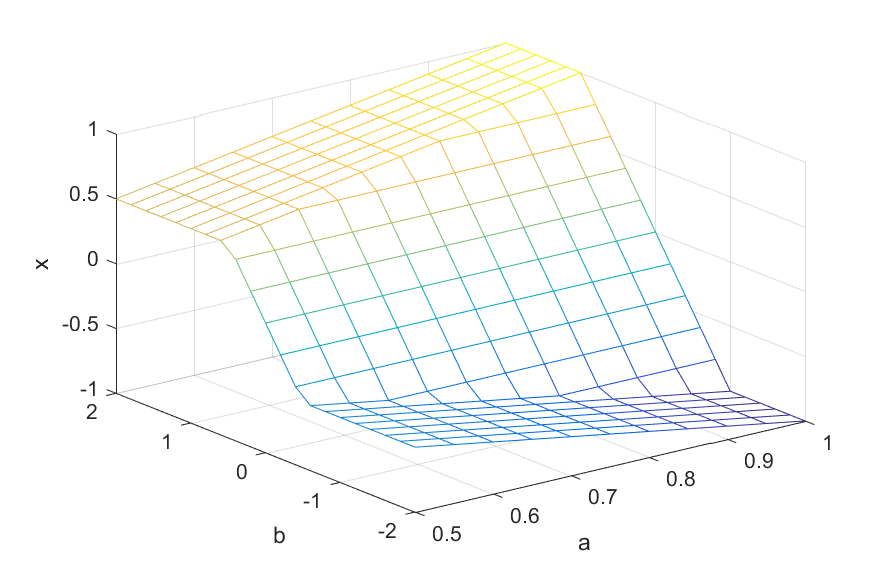
Let us use this partial instantiation to plot the optimal \(x\) as a function of \(a\) and \(b\) over a grid (we’ll show below how you can do this quicker without this new partial instantiation, this is just for illustration)

Saturation = optimizer([-a <= x <= a ], Objective,sdpsettings('solver','mosek'), { a , b}, x);
% Create a grid
[A,B] = meshgrid(0.5:0.05:1,-2:0.2:2);
for i = 1:size(A,2)
    Saturation_fixeda = Saturation(A(1,i),[]);
    for j = 1:size(A,1)        
        Optimal(j,i) =  Saturation_fixeda(B(j,i));
    end
end
mesh(A,B,Optimal);
xlabel('a');ylabel('b');zlabel('x')

Alternatively

for i = 1:size(A,2)
    for j = 1:size(A,1)        
        Optimal(j,i) =  Saturation(A(j,i),B(j,i));
    end
end
mesh(A,B,Optimal);

Fastest approach is a blocked augmentation of multiple arguments. The first line of code below compiles and solves 231 quadratic programs over a grid!

Optimal = Saturation(A(:)',B(:)');
mesh(A,B,reshape(Optimal,size(A)));

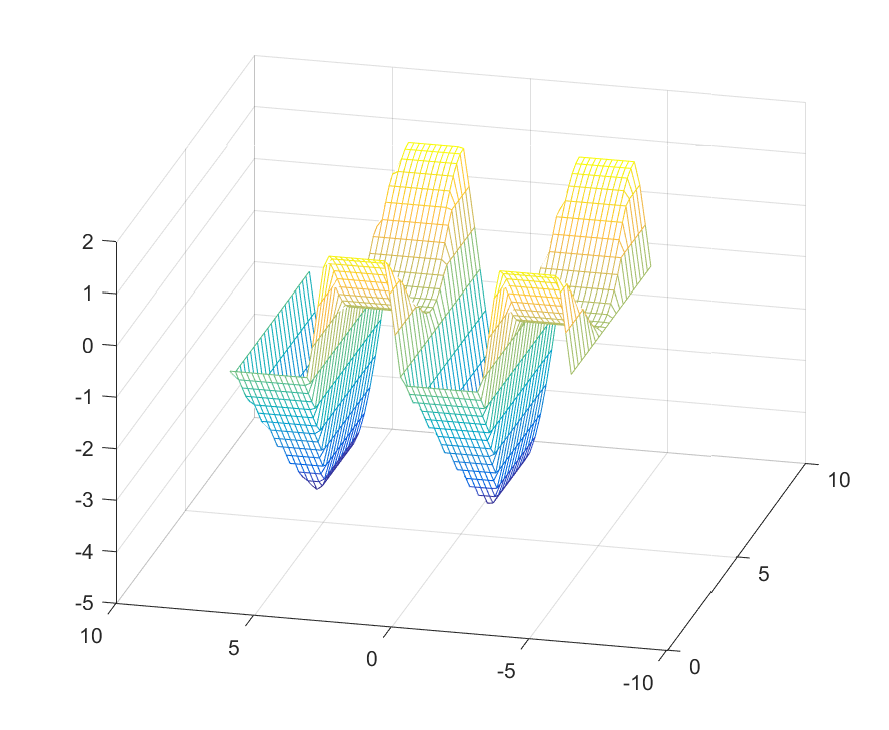
Remember, optimizer is not just for linearly parameterized problems or simple quadratic programs. However, when there are general callback nonlinearities acting on parameters (functions such as exp, log etc), they can (currently) only act on simple parametric variables, i.e., not on any kind of compound expression involving parameters. Note that the problem below is a nonlinear program for YALMIP during the compilation phase, and is a quadratic program first when the parameters have been fixed. It is thus a case where it is crucial that we explicitly select a suitable solver for the instantiated problem.

Objective = (x-4*sin(b))^2;
Saturation = optimizer([-a <= x <= 1 + cos(a) ], Objective,sdpsettings('solver','mosek'), { a , b}, x);
[A,B] = meshgrid(0.5:0.25:2*pi,-2*pi:0.2:2*pi);
Optimal = Saturation(A(:)',B(:)');
mesh(A,B,reshape(Optimal,size(A)));

Delayed solution and concatenation of optimizer objects

We can perform a full parameterization, but delay the solution of the optimization problem

Solver = saturation(1,3,'nosolve');

xoptimal = Solver([]);

This feature can be useful in some cases where we concatentate several models, and then solve a problem on the intersection of all constraints.

Another new feature is the possibility to concatenate optimizer objects. This is in particular useful when performing partial instantiations. All constraints in the concatenated models are appended, and the new objective is the average of all involved objectives, i.e, they are summed up.

Consider a case where we have two models

Objective = (x - b + a)^2;
Saturation = optimizer([-a-b <= x <= a+b ], Objective,sdpsettings('solver','mosek'), { a , b}, x);

Case1 = Saturation(a == 1);
Case2 = Saturation(a == 2);

Merge = [Case1,Case2];
xoptimal = Merge(1)

Effectively, we just solved

xoptimal = optimize([-1-1 <= x <= 1+1,-2-1 <= x <= 2+1],((x-1+1)^2+(x-1+2)^2)/2)

An alternative here is to use a delayed solve, and fully instantiate all objects before merging them.

Case1 = Saturation(a == 1, b==1,'nosolve');
Case2 = Saturation(a == 2, b==1,'nosolve');
Merge = [Case1,Case2];
xoptimal = Merge()

Note that current relase assumes that all concatenated models involve exactly the same variables, both parameters and decision variables.