Sample-based robust optimization

By using partially instantiated optimizer objects, we can build a sceanrio-based robust optimization solver.

Defining a ball as an uncertain linear constraint

To illustrate the ideas, we will start with some basic YALMIP code to show how a circle can be approximated using hyperplanes, i.e., we will create a polytopic outer approximation.

The ball \(x^Tx \leq 1\) can alternatively be written as \(v^Tx \leq 1 ~\forall ~v^Tv\leq 1 \) (the dual-norm property). Hence, the following lines of code generate a ball approximation and plots it together with the exact ball (we sample \(v\) on the unit-circle as samples inside in the interior will generate redundant constraints)

x = sdpvar(2,1);
ballApproximation = [];
for i = 1:10
 v = randn(2,1);v = v/norm(v);
 ballApproximation = [ballApproximation, v'*x <= 1];
end
clf
plot(ballApproximation,x,'blue');hold on
plot(x'*x <= 1,x,'red');

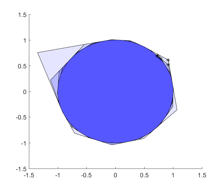
Let us see how this approximation evolves as we increase the number of hyperplanes, and let us also solve an optimization problem where we maximize \(x_1+x_2\) over the approximation just to see how this solution converges.

x = sdpvar(2,1);
ops = sdpsettings('plot.shade',.1,'verbose',0);
ballApproximation = [];
clf;hold on
for k = 1:10
  for i = 1:10
    vi = randn(2,1);vi = vi/norm(vi);
    ballApproximation = [ballApproximation, vi'*x <= 1];
  end
  plot(ballApproximation,x,'blue',200,ops);
  optimize(ballApproximation,-sum(x),ops);  
  plot(value(x(1)),value(x(2)),'k*');drawnow
end 

In the plot command, we use 200 rays to increase the likelihood of not missing any vertices during ray-shooting. In other words, the code above solves 2000 linear programs to plot the sequence of ball approximations, so you better have an efficient solver installed (code takes around 10-15 seconds with a quality linear programming solver installed).

Optimizer to the rescue

In a first step to use the recent additions to YALMIP optimizer objects, we use partially instantiated optimizer objects. We want to generate a bunch of constraints with different \(v\) but the same \(x\). Hence, we create a model which is parameterized in \(v\), and then instantiate objects where \(v\) is fixed to different values, and concatenate these. Conveniently, plot is overloaded on optimizer objects and simply plots the feasible set in any remaining decision- or parametric variables. Note that the uninstantiated model is bilinear in the variables, hence it is crucial to specify a solver which is applicable once the parameters have been fixed. Also note the use of the flag ‘nosolve’ which stops the optimizer object from solving the instantiated model

x = sdpvar(2,1);
v = sdpvar(2,1);
ops = sdpsettings('plot.shade',.1,'verbose',0,'solver','mosek');
ballApproximation = [];
paramModel = optimizer(v'*x <= 1,-sum(x),ops,v,x);
clf;hold on
for k = 1:10
  for i = 1:10
    vi = randn(2,1);vi = vi/norm(vi);
    ballApproximation = [ballApproximation, paramModel(vi,'nosolve')];
  end
  plot(ballApproximation,x,'blue',200,ops);
  xopt = ballApproximation();
  plot(xopt(1),xopt(2),'k*');
  drawnow
end 

Generic uncertainty sets and sampling based scenarios through optimizers

The command uncertain has previously been used for declaring uncertain variables in a robust optimization problem, which then has been solved using derivations of worst-case robust counterparts. It is now possible to attach a distribution or sample generator to an uncertainty declaration of a parameter used in an optimizer.

In the distribution case (other cases below), we specify a distribution with associated parameters from the list of distributions available in the random command (random is part of the Statistics Toolbox).

The following specifies a model where all elements in v are random variables with uniform distribution between \(-1\) and \(1\)

Model = [v'*x <= 1, uncertain(v,'unif',[-1;-1],[1;1])];

YALMIP automatically appends dimension information to the call to random, which means random automatically generates samples of correct dimension if you give scalar distribution parameters

Model = [v'*x <= 1, uncertain(v,'unif',-1,1)];

It is important that you supply all parameters for the distribution, as YALMIP always appends dimensions as trailing arguments, and if you omit some parameter, the dimension arguments will be interpreted as distribution parameters by random.

Create an optimizer with a parameter which has a distribution definition.

Model = [v'*x <= 1, uncertain(v,'unif',[-1;-1],[1;1])];
OneHyperPlaneModel = optimizer(Model, -sum(x),ops,v,x);

We can instantiate this model as usual for a particular value on v.

model = OneHyperPlaneModel([-1;1],'nosolve');

However, we can also tell it to draw samples on parameters with distributions attached, and instantiate the object using those values instead.

model = sample(OneHyperPlaneModel)

To create a model with several cuts, we simply concatenate the samples

model = sample(OneHyperPlaneModel);
for i = 1:10
  model = [model, sample(OneHyperPlaneModel)];
end

This can be simplified, and we can tell the sampler to draw several samples in one call, and concatenate those models.

model = sample(OneHyperPlaneModel,10);

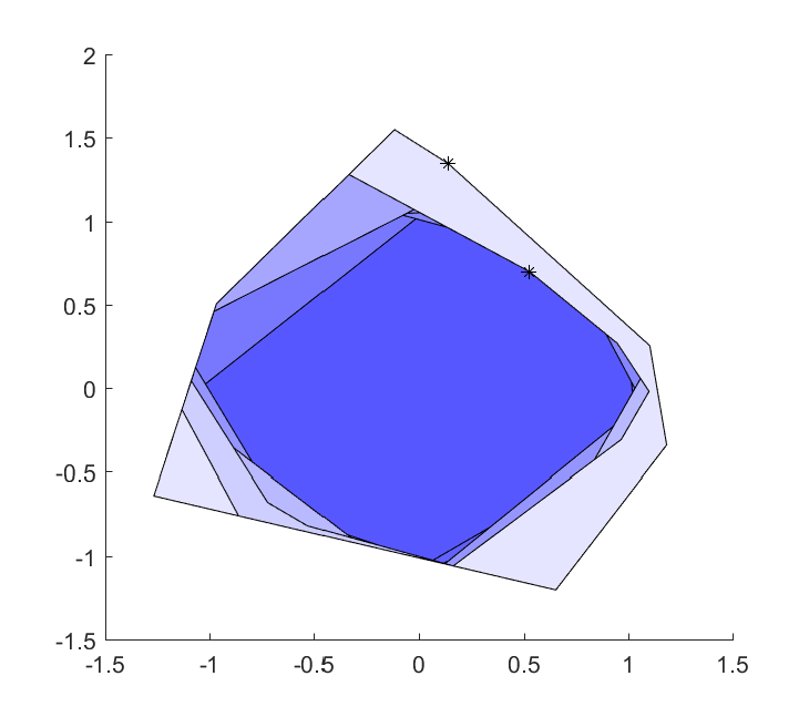
Now that we can attach a distribution to a variable, and sample models, let us put this to use. In our first experiment, we will not reproduce the figure above, but create the set \(v^Tx \leq 1 ~\forall ~\left\lvert v \right\rvert \leq 1 \). If you’ve done your homework, you should already now realize that will create a romb (asymptotically). Note that rombApproximation will be an optimizer object without any remaining parameters. To execute a solve, we simply give it an empty list of parametric values.

x = sdpvar(2,1);
v = sdpvar(2,1);
ops = sdpsettings('plot.shade',.1,'verbose',0,'solver','mosek');
rombApproximation = [];
Model = [v'*x <= 1, uncertain(v,'unif',-1,1)];
Model = optimizer(Model,-sum(x),ops,v,x);
clf;hold on
for k = 1:10
  rombApproximation = [rombApproximation, sample(Model,10)];  
  plot(rombApproximation,x,'blue',200,ops);
  xopt = rombApproximation();
  plot(xopt(1),xopt(2),'k*');drawnow
end 

As we sample in the whole set (as in contrast to the boundary), we are generating a lot of redundant constraints.

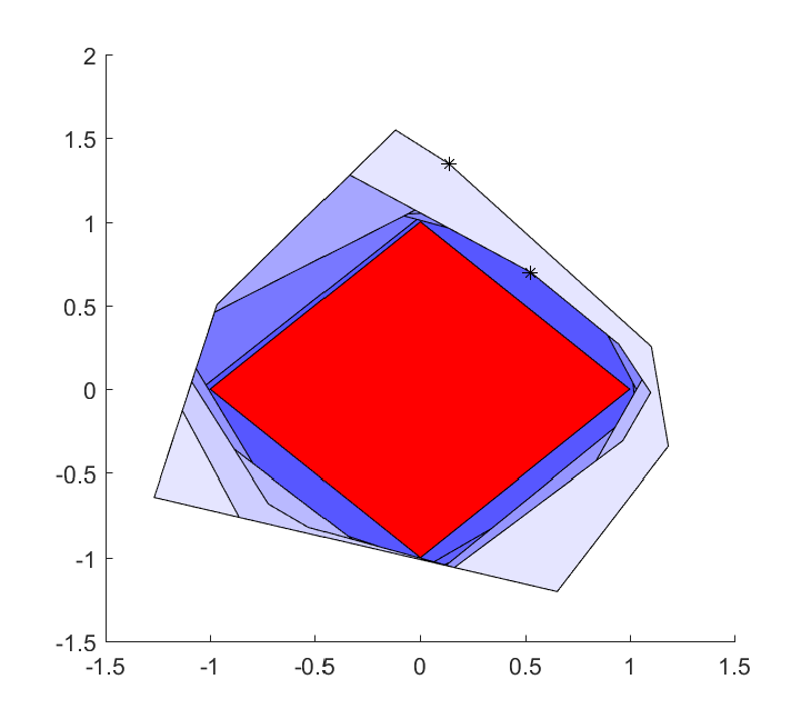
Of course, this is a silly way to specify the set \(\left\lvert v \right\rvert \leq 1 \). An alternative old-school YALMIP approach to create this set in a silly way is to create it using the deterministic exact worst-case robust optimization framework, where the dual norm property is automatically derived (leading to a model with ony four linear constraints)

Model = [v'*x <= 1, uncertain(-1 <= v <= 1)];
plot(Model,x,'red');

The reason we started playing with an approximation of a romb, instead of the original ball approximation, is that there is no distribution in the random command which samples on the bounded unit ball. What we can do instead is to attach the variable with a general function handle which generates a sample of suitable character.

We create a function which creates samples on the unit circle

% mysampler.m
function z = mysampler(dim)
z = randn(dim(1),1);z = z/norm(z);

This sampler can now be assigned to an uncertain variable

Model = [v'*x <= 1, uncertain(v,@mysampler)];

Note that the sampler always sends the variable dimension to the sampler, which thus can be used in our function. If we have more arguments in our sample creater, we must specify those arguments

% mysampler.m
function z = mysampler(center, dim)
z = randn(dim(1),1);z = center + z/norm(z);

````matlab
Model = [v'*x <= 1, uncertain(v,@mysampler,[0;0])];

Using anonymous function on-the-fly is also an alternative

f = @(dim)randn(dim(1),1);g = @(x)(x/norm(x));
ball = @(x)g(f());

At this point, we are ready to regenerate the plot of the ball approximation.

x = sdpvar(2,1);
v = sdpvar(2,1);
ops = sdpsettings('plot.shade',.1,'verbose',0,'solver','mosek');
ballApproximation = [];

f = @(x)randn(2,1);g = @(x)(x/norm(x));
ballSampler = @(x)g(f());

Model = [v'*x <= 1, uncertain(v,ballSampler)];
Model = optimizer(Model,-sum(x),ops,v,x);
clf;hold on
for k = 1:10
  ballApproximation = [ballApproximation, sample(Model,10)];  
  plot(ballApproximation,x,'blue',200,ops);
  xopt = ballApproximation();
  plot(xopt(1),xopt(2),'k*');drawnow
end 

This generalizes almost arbitrarily (well, limited by the current implementation of optimizer where better support for nonlinear calback is needed). Nothing forces us to have models linear in the random variables, nor do we have to have simple balls in which the uncertainty lives.

x = sdpvar(2,1);
v = sdpvar(2,1);
ops = sdpsettings('plot.shade',.1,'verbose',0,'solver','mosek');
setApproximation = [];

f = @(x)randn(2,1);g = @(x)(sin(x)/(1 + abs(sum(x))/5));
weirdSampler = @(x)g(f());

Model = [v'*x <= 1 + sum(v.^4-v.^3), uncertain(v,weirdSampler)];
Model = optimizer(Model,-sum(x),ops,v,x);
clf;hold on
for k = 1:20
  setApproximation = [setApproximation, sample(Model,10)];  
  plot(setApproximation,x,'blue',200,ops);
  xopt = setApproximation();
  plot(xopt(1),xopt(2),'k*');drawnow
end 

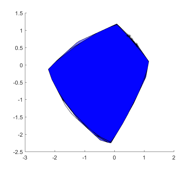
Note that the resulting sets are all convex, as they are intersections of convex sets (hyperplanes), regardless of how complex the sampling is, or how the uncertainty enters the model.