Robust optimization

The robust optimization module is described in the paper Löfberg 2012 (which should be cited if you use this functionality). Small errata.

Background

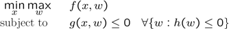
In a general setting, robust optimization deals with optimization problems with two sets of variables, decision variables (here denoted x) and uncertain variables (w). The goal in deterministic worst-case robust optimization is to find a solution on the decision variables such that the worst-case cost is minimized and the constraints are robustly feasible, when the uncertainty is allowed to take arbitrary values in a defined uncertainty set.

YALMIP cannot deal with arbitrary uncertain problems (it is in general an intractable problem), but focus on special cases.

Supported scenarios

The different cases are called scenarios in the paper above, and they are converted to a robust counterpart using so called filters. There are three major scenarios with corresponding filters, all discussed in the paper referenced above.

1. For elementwise constraints \(b^Tx + (A^Tx + c)^Tw\leq 0\) (affinely parameterized in the uncertainty for fixed x), polytopic and general conic uncertainty sets are supported. The uncertainty is eliminated using either duality theory or enumeration. For the enumeration approach to work, you must have MPT installed.

2. For elementwise constraints \(b^Tx + (A^Tx + c)^Tw\leq 0\) and the uncertainty constrained to a norm-ball (\(p=1,2,\infty\)), the uncertainty is removed by explicitly maximizing the expression w.r.t the uncertainty typically leading to a very efficient representation of the worst-case.

3. For conic constraints affinely parameterized in the uncertainty, polytopic uncertainty sets are supported. The uncertainty is removed using enumeration.

In addition to these three major scenarios, there are some less general approaches.

1. If the uncertainty enters polynomially and the uncertainty lives on a standard simplex, a conservative robust counterpart, based on Polya’s relaxation, is used.

2. If the uncertainty enters affinely (for fixed x) and the uncertainty is constrained by a conic set, a conservative sum-of-squares based approach is used.

Simple linear programming examples

Let us begin with a trivial problem with a scalar decision variable x and a scalar uncertainty w. We create a problem with one uncertain constraint, and a simple uncertainty model.

sdpvar x w
F = [x+w <= 1];
W = [-0.5 <= w <= 0.5, uncertain(w)];
objective = -x;

Obviously, the optimal maximal x is 0.5, since if x is larger, there exist a w such that the uncertain constraint is violated.

To solve the problem, we call optimize. A robust counterpart will automatically be derived and solved (generally, linear constraints with polytopic uncertainty is dealt with using the enumeration approach referenced above, however, for simple box uncertainty as in this case, YALMIP explictly performs the maximization, leading to a more efficient worst-case model)

sol = optimize(F + W,objective)

An alternative (which does not simplify anything here) is to model the uncertainty using a convex hull model, i.e. parameterize the uncertainty in terms of vertices. Note that we have to add the auxiliary variables t1 and t2 to the list of uncertain variables, since there is no way for YALMIP to figure out that these variables are used to describe the uncertainty.

sdpvar x w t1 t2
F = [x+w <= 1];
W = [w == t1*(-0.5) + t2*0.5, t1+t2 == 1, 0 <= [t1 t2] <= 1]
W = [W,uncertain([t1 t2 w])];
objective = -x;
sol = optimize(F + W,objective)

In this case, the explicit norm-ball filter cannot be invoked, and the enumeration filter is used. If you want to try the duality filter, simply change an option

sdpvar x w t1 t2
F = [x+w <= 1];
W = [w == t1*(-0.5) + t2*0.5, t1+t2 == 1, 0 <= [t1 t2] <= 1]
W = [W,uncertain([t1 t2 w])];
objective = -x;
sol = optimize(F + W,objective,sdpsettings('robust.lplp','duality')

Conic uncertainty models

The uncertainty description has to be conic representable (which in YALMIP means that it only uses linear conic constraints, or [nonlinear operators] that can be represented using linear conic constraint).

The following more advanced model should have an optimal objective of 0.

sdpvar x w(2,1)
F = [x+sum(w) <= 1];
W = [norm(w) <= 1/sqrt(2), uncertain(w)];
objective = -x
sol = optimize(F + W,objective)

The following alternative model is also valid.

sdpvar x w(2,1)
F = [x+sum(w) <= 1];
W = [w'*w <= 1/2, uncertain(w)];
objective = -x
sol = optimize(F + W,objective)

More advanced problems

The robustification is done using strong duality arguments in the uncertainty space, or by simple enumeration. This means that there is no problem with integer and logic constraints in the decision variables

sdpvar x w
F = [x+w <= 1, ismember(x,[0.2 0.4])];
W = [-0.5 <= w <= 0.5,uncertain(w)];
objective = -x;
sol = optimize(F + W,objective)

To illustrate even stronger how transparently integrated the robust optimization framework is, we solve an uncertain [sum-of-squares] problem involving a [nonlinear operator] leading to integrality constraints, thus forcing the resulting SDP to be solved using the internal mixed-integer SDP solver BNB.

We want to find an integer value \(a\), taking values in the range from 3 to 5, such that the polynomial \(ax^4+y^4+uxy+1\) has a lower bound larger than \(t\), for any \(-1 \leq u\). A trivial and contrived example of course, but here is the compact YALMIP model.

sdpvar x y t u a

p = a*x^4+y^4+u*x*y+1;

F = [uncertain(u), -1 <= u <= 1];
F = [F, ismember(a,[3 4 5])];
F = [F, sos(p - t)];

solvesos(F,-t)

Uncertain semidefinite and second order cone constraints

YALMIP can robustify second order cone (SOCP) and semidefinite (SDP) constraints with affine dependence on the uncertainty, under the restriction that the uncertainty is constrained to a polytopic set. In this case, YALMIP derives a robust counterpart by enumerating the vertices of the uncertainty set and define a new SOCP or SDP constraint for every vertex. For the enumeration to work, you have to have MPT installed.

The following code computes a common Lyapunov function for a system with uncertain dynamics.

t = sdpvar(1,1);
P = sdpvar(2,2);
A = [-1 t;0.2 -1]

F = [A'*P + P*A <= -eye(2), 1 <= t <= 2, uncertain(t)];
sol = optimize(F,trace(P))

For more examples, check out the LPV control example

Useful features

In some cases, we only want to derive the robust counter-part, but not actually solve it. This can be accomplished with the command [robustify]

[Frobust,robust_objective] = robustify(F + W,objective);

The robustified model can be manipulated as any other YALMIP model and can of course be solved

sol = optimize(Frobust,robust_objective);