Model predictive control - LPV models
This example, contributed by Thomas Besselmann, accompanies the paper Besselmann and Löfberg 2008)
Note that the code below uses some awkward, no longer necessary, reformulations in order to cope with uncertainty in linear programming representable nonlinear terms.
Introduction
We consider linear discrete-time LPV systems with a parameter-varying state transition and parameter-varying input matrix

This allows one to model systems, where the system dynamics depend on scheduling signals, and this scheduling signal is measurable, but not known in advance.
When the input matrix B is constant, a simpler scheme can be used, which is demonstrated in the LPVA-MPC example.
Explicit MPC for LPV systems
Let us find the explicit solution to a variant of the MPC problem for LPV systems. This will be a pretty advanced example, so let us start slowly by defining some data.
% YALMIP options
yalmip('clear')
yopts = sdpsettings('robust.polya',1);

% Model data
A1 = [0.85 0;0.25 0.65];
A2 = [0.85 0;-0.3 0.65];
B1 = [1;-1];
B2 = [1;1];
B{1} = B1;
B{2} = B2;

% System sizes
nx   = 2; % Number of states
nu   = 1; % Number of inputs
ndyn = 2; % Number of vertex systems

% State and input constraints
xmin = [-10;-10];
xmax = [  8;  8];
umin = -0.5;
umax =   1 ;

% MPC data
Q   = eye(nx);
R   = 0.01;
N   = 3;
xref = [0;0];
With robust.polya, the degree of the Pólya relaxation is defined. It converges asymptotically to the true problem with increasing Pólya degree. The used norm in this example is the infinity-norm. To simplify the code and the notation, we create state, control and scheduling parameters in cell arrays.
% States x(k), ..., x(k+N)
x = sdpvar(repmat(nx,1,N),repmat(1,1,N));
% Inputs u(k), ..., u(k+N) (last one not used)
u = sdpvar(repmat(nu*ndyn,1,N),repmat(1,1,N));
% Scheduling parameter
th = sdpvar(repmat(ndyn,1,N),repmat(1,1,N));
% Epigraph variable
sdpvar w;
Dynamic Programming Iterations
Now, instead of setting up the problem for the whole prediction horizon, we only set it up for one step, solve the problem parametrically, take one step back, and perform a standard dynamic programming value iteration.
for k = N:-1:1   % shifted: N-1:-1:0

    % Parameter simplex
    F = [uncertain(th{k}), sum(th{k}) == 1, 0 <= th{k} <= 1];
    % Epigraph variable, MPT requires a bounded set so let us add artificial upper bound
    F = [F, 0 <= w <= 10000];

    % Uncertain predictions and control
    uth = kron(th{k},eye(nu))'*u{k};    % u(th)
    Ath = [A1 A2]*kron(th{k},eye(nx));  % A(th) = A1*th1 + A2*th2 + ...
    Bth = [B1 B2]*kron(th{k},eye(nu));  % B(th)
    xp  = Ath*x{k} + Bth*uth;

    % Input constraints
    F = [F, repmat(umin,ndyn,1) <= u{k} <=  repmat(umax,ndyn,1)];

    % State constraints
    F = [F, xmin  <= x{k} <= xmax];

    % Insert step-specific code here
    if k == N
     % Initial step
    elseif k > 1
     % Intermediate step
    else
     % Final step
    end

    % Determine robust counterpart
    [F,obj] = robustify(F,obj,yopts,th{k});

    % Solve multi-parametric problem
    [sol{k},diagnost{k},Uz{k},J{k},Optimizer{k}] = solvemp(F,obj,yopts,x{k},u{k});
end
In the first and the last step of the iteration, some parts of the code differ from the remaining steps. The common parts are the definition of the parameter simplex, the state update equation, the state and input constraints, the robust counterpart and the solution of the resulting multi-parametric program. In the following the step dependent code snips are listed.
First step
In the first step we rewrite the inf-norm into an epigraph formulation, and add constraints for the final state. Note that we have to manually derive the epigraph models of the sum-of-inf-norms (this is no longer the case, this is from an old YALMIP version)
% |x| written as max(a[x;u]+b)
a = [kron(eye(nx),[1 -1]') zeros(2*nx,nu)];
b = zeros(2*nx,1);
% |u| written as max(c[x;u]+d)
c = [zeros(2*nu,nx) kron(eye(nu),[1 -1]')];
d = zeros(2*nu,1);

% |x|+|u| written as max(aa[x;u]+bb)
aa = repmat(a,2*nu,1) + kron(c,ones(size(a,1),1));
bb = repmat(b,2*nu,1) + kron(d,ones(size(a,1),1));

% Final state constraints
F = [F, xmin  <= xp   <= xmax];

% Cost function
F   = [F, aa*[Q*(xp-xref);R*uth]+bb + norm(Q*(x{k}-xref),inf) <= w];
obj = w;
Intermediate steps
In the following steps we get the hyperplanes from the previous solution for the cost-to-go. We constrain the predicted states to be a feasible state for the preceding step of the DP iteration.
% Get the hyperplanes for cost-to-go
S = unique(([reshape([sol{k+1}{1}.Bi{:}]' ,nx,[])'  reshape([sol{k+1}{1}.Ci{:}]' ,[],nu)]),'rows');
a = [S(:,1:nx) zeros(size(S,1),nu)];
b = S(:,nx+1:end);

% Jp+|u| = max(a[x;u]+b)+|u|=max(a[x;u]+b)+max(c[x;u]+d)=max(aa[x;u]+bb)
aa = repmat(a,2*nu,1) + kron(c,ones(size(a,1),1));
bb = repmat(b,2*nu,1) + kron(d,ones(size(a,1),1));

% Constrain predicted state
[H,K] = double(sol{k+1}{1}.Pfinal);
F     = [F, H*xp <= K];

% Cost function
F   = [F, aa*[xp;R*uth]+bb <= w];
obj = norm(Q*(x{k}-xref),inf) + w;
Final step
In the last step we use the uncontrolled successor step to improve control performance. The code snip inserted into the iteration is:
% Get the hyperplanes for cost-to-go
S = unique(([reshape([sol{k+1}{1}.Bi{:}]',nx,[])' reshape([sol{k+1}{1}.Ci{:}]',[],nu)]),'rows');
a = [S(:,1:nx) zeros(size(S,1),nu)];
b = S(:,nx+1:end);

% Jp+|u| = max(a[x;u]+b)+|u|=max(a[x;u]+b)+max(c[x;u]+d)=max(aa[x;u]+bb)
aa = repmat(a,2*nu,1) + kron(c,ones(size(a,1),1));
bb = repmat(b,2*nu,1) + kron(d,ones(size(a,1),1));

% State update equation
xp = x{k} + Bth*uth; % x{1} = z

% Constrain predicted state
[H,K] = double(sol{k+1}{1}.Pfinal);
F     = [F, H*xp <= K];

% Cost function
F   = [F, aa*[xp;R*uth]+bb <= w];
obj = w;

% add eps-penalty on vertex predictions
for v = 1:ndyn
    xpv{v} = x{k} + B{v}*u{k}(v);
    obj = obj + 0.001*norm(Q*xpv{v},inf);
end
Results
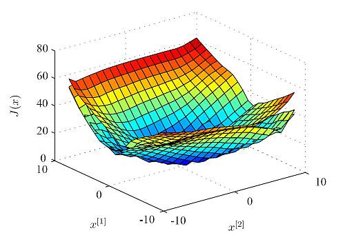
Finally the control performance of the Explicit LPV-MPC controller is compared to robust control and the truely optimal solution for a certain scheduling parameter trajectory (for details see the above mentioned paper). The actual costs of the closed-loop system over a grid of initial points are depicted in the following Figure. While Explicit LPV-MPC performs in average only 0.4 % worse than the truely optimal solution, robust MPC leads to an average of 23.3 % increase of the actual costs.
The resulting explicit LPV-MPC controller takes the scheduling parameter into account, and thus outperforms robust MPC. Nevertheless, it is an explicit MPC controller, and enables constrained gain-scheduling control at high sampling rates, which is not possible for the truely optimal solution.
