State feedback design for LPV system
This example illustrates an application of the robust optimization module. The main focus of this example is uncertain semidefinite constraints.
In addition to the robustification of linear constraints, introduced in the robust MPC example, YALMIP can also robustify second-order cone and semdefinite constraints bilinear in the decision variable and the uncertainty.
Robust control
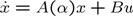
Our goal is to compute a controller \(u=Kx\) for an uncertain linear system.
The performance measure is given by the standard infinite horizon quadratic cost
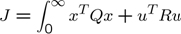
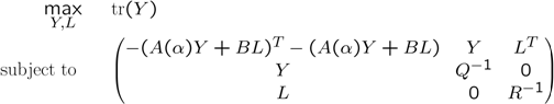
A controller which minimizes the worst case cost is given by solving the following semidefinite programming problem.

This is a nonconvex problem, but a standard trick in control Boyd et al. 1994 is to perform a congruence transformation with \(Y=P^{-1}\), introduce \(L=KY\), and apply a Schur complement. Instead of solving the nonconvex problem, the following problem is solved instead (never mind the odd change of objective)
Let us now solve a problem of this type for a system with a polytopic \(A\) matrix. Define the nominal model.
Anominal = [0 1 0;0 0 1;0 0 0];
B = [0;0;1];
Q = eye(3)
R = 1;
Manual implementation
The uncertainty we will address is a perturbation in the (1,3) element. We create two matrices to denote the two extreme values of the uncertain matrix.
A1 = Anominal;A1(1,3) = -0.1;
A2 = Anominal;A2(1,3) =  0.1;
Before we employ the automatic support for robust semidefinite programming, note that this is the manually derived worst-case problem and solution (The tag ‘full’ is used here to remind novel users that for variables that should be fully parameterized, use the tag. It is a common mistake to copy code and then all of a sudden when the matrix is square, you forget to add the tag ‘full’ and get a symmetric matrix. See basic.)
Y = sdpvar(3,3);
L = sdpvar(1,3,'full');

F = [Y >= 0];
F = [F, [-A1*Y-B*L + (-A1*Y-B*L)' Y L';Y inv(Q) zeros(3,1);L zeros(1,3) inv(R)] >= 0];
F = [F, [-A2*Y-B*L + (-A2*Y-B*L)' Y L';Y inv(Q) zeros(3,1);L zeros(1,3) inv(R)] >= 0];
optimize(F,-trace(Y))
K = value(L)*inv(value(Y));
Semi-manual implementation
Now let us do this using the robust optimization module. Define the uncertain system,
sdpvar t1 t2
A = A1*t1 + A2*t2;
the uncertain semidefinite constraint (note that it is parameterized in the uncertain variables t1 and t2),
F = [Y >=0];
F = [F, [-A*Y-B*L + (-A*Y-B*L)' Y L';Y inv(Q) zeros(3,1);L zeros(1,3) inv(R)] >= 0];
and the uncertainty description
F = [F, 0 <= [t1 t2] <= 1, t1+t2 == 1, uncertain([t1 t2])];
Finally, we solve the uncertain problem using optimize.
optimize(F,-trace(Y))
The optimal feedback can be recovered
K = value(L)*inv(value(Y))
Fully automatic implementation
For this simple case with only two vertices, and with the two vertices given, the manual code is almost easier, but the benefit is obvious when the parameterization is more complex and there are several uncertainties.
The model above is derived semi-manually, since we worked explicitly with the vertices of the A matrix. An alternative approach is to simply parameterize the matrix.
What we would like to do is the following:
alpha = sdpvar(1);
A = Anomial;
Anominal(1,3) = alpha;
Unfortunately, this will fail, due to limitations in MATLABs overloading of assignment of user-defined classes. Instead, we have to use the following approach
alpha = sdpvar(1);
A = [0 1 alpha;0 0 1;0 0 0];
We have now created a parameterized system, and can proceed as before.
F = [Y >=0];
F = [F, [-A*Y-B*L + (-A*Y-B*L)' Y L';Y inv(Q) zeros(3,1);L zeros(1,3) inv(R)] > 0]

F = [F, -0.1 <= alpha <= 0.1, uncertain(alpha)];

optimize(F,-trace(Y))

K = value(L)*inv(value(Y))
Gain scheduling control
As a second slightly more advanced example, we extend the problem to gain scheduling. We now assume that the uncertain parameter is unknown at design time, but known on-line. This means we can make the controller depend on the uncertainty.
Parameterized feedback matrix
Since there is no uncertainty in \(B\), and \(L\) only enter linearly or in products with \(B\), we can parameterize \(L\).
L0 = sdpvar(1,3);
L1 = sdpvar(1,3);

L = L0 + alpha*L1;
The constraints are still bilinear in uncertainty and decision variables, i.e. linear in the uncertainty, so we can solve the worst-case problem in the same way as above.
F = [Y >=0];
F = [F, [-A*Y-B*L + (-A*Y-B*L)' Y L';Y inv(Q) zeros(3,1);L zeros(1,3) inv(R)] >= 0)];
F = [F, -0.1 <= alpha <= 0.1, uncertain(alpha)];
optimize(F,-trace(Y))
You should notice that the objective value is not improved, hence the parameterization did not help.
Parameterized feedback matrix and Lyapunov matrix
As a final example, let us try to make the controller less conservative by parameterizing also the Lyapunov matrix \(Y\). Unfortunately, this is a bit trickier. Since there are products between the uncertain matrix \(A\) and the \(Y\), the uncertainty will possibly enter the problem nonlinearly.
However, since the uncertainty only enter \(A\) in the (1,3) element, it is easily seen that the following parameterization will yield no nonlinear uncertainties terms in the product between \(A\) and \(Y\).
Y0 = sdpvar(3,3);
Y1 = sdpvar(3,3);

Y1(:,3) = 0;
Y1(3,:) = 0;

Y = Y0 + alpha*Y1;
this can easily be checked
degree(A*Y,alpha)

ans =

     1
Solve the problem once again, now with parameterized feedback matrix and Lyapunov matrix (notice the larger objective value, which is a result of a less conservative problem formulation)
F = [Y >=0];
F = [F, [-A*Y-B*L + (-A*Y-B*L)' Y L';Y inv(Q) zeros(3,1);L zeros(1,3) inv(R)] >= 0]
F = [F, -0.1 <= alpha <= 0.1, uncertain(alpha)];
optimize(F,-trace(Y))
This step where we used a reduced parameterization to avoid products between uncertainties can easily be automated, and this is actually implemented in YALMIP. Hence, we can define a full parameterization, and YALMIP will automatically derive constraints on the decision variables such that no nonlinear uncertainty terms occur, if possible.
Y0 = sdpvar(3,3);
Y1 = sdpvar(3,3);
Y = Y0 + alpha*Y1;

F = [Y >= 0];
F = [F, [-A*Y-B*L + (-A*Y-B*L)' Y L';Y inv(Q) zeros(3,1);L zeros(1,3) inv(R)] >= 0]
F = [F, -0.1 <= alpha <= 0.1, uncertain(alpha)];
optimize(F,-trace(Y))
