MAXPLUS control

This example illustrates how control based on max-plus algebra can be implemented in YALMIP, by relying on automatic convexity analysis and the overloaded max operator.

If you are unfamiliar with max-plus control and tropical algebra, an introduction to the max-plus control problem can be found in this report by B. De Schutter and T. van den Boom, whereas a more detailed mathematical background to tropical algebra can be found in this mini-course by Stéphane Gaubert.

Max-plus algebra

The max-plus, or tropical, algebra is an algebra where there are two operators, tropical addition and tropical multiplication.

For scalar arguments, the tropical addition is nothing but the maximum of its arguments, and tropical multiplication is standard addition.

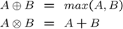
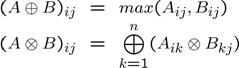
The generalization to the matrix case is defined as follows.

We note that tropical addition already is available in YALMIP, since the max operator, with convexity and monotonicity knowledge, is overloaded on matrix variables, via the [nonlinear operator framework]. The tropical multiplication however requires some code for the matrix case. To simplify coding, a command ttimes is available.

function C = ttimes(A,B)

n = size(A,1);
m = size(B,2);
X = kron(ones(m,1),A);
Y = kron(B',ones(n,1));
C = reshape(max(X+Y,[],2),n,m);

For consistency, a command tplus is also available.

function C = tplus(A,B)

C = max(A,B);

Max-plus control

Max-plus control means control of systems where the state-update equations, and possibly also constraints and objective functions, are allowed to contain max-plus expressions.

In a YALMIP context, there is nothing special with a max-plus system. It is simply a special case of a system where the state update equations are allowed to contain [Tutorials.nonlinearOperators nonlinear operators] such as max, min, abs, sumk etc.

The purpose of this example is not to advocate YALMIP as a tool for solving max-plus control problems, but to illustrate that max-plus control falls into the general framework of YALMIP with very little additional coding (all we have to do is to define the tplus and ttimes operators)

Since YALMIP automatically propagates convexity knowledge, convex cases are automatically detected and solved efficiently. In the max-plus community, one proposed approach to solve nonconvex cases is to apply so called extended complementarity algorithms, whereas YALMIP will formulate the nonconvex cases using binary variables and solve the problem using mixed integer programming.

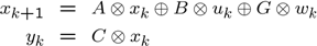
A linear max-plus system is obtained by simply changing addition and multiplication to the tropical counterparts.

It follows directly from [Tutorials NonlinearOperators convexity rules and properties of \(max\)] that future states and outputs are convex in the current state and control inputs, if the \(A\), \(B\) and \(C\) matrices only have non-negative elements.

In MPC, a performance objective is minimized subject to constraints on future states, outputs and inputs.

Once again, directly from the convexity propagation rules, the MPC problem is convex if the stage-cost \(L\) and the constraint\(g\) is convex and non-decreasing.

The issue we want to emphasize here is that YALMIP automatically detects these properties and sets up a corresponding convex optimization problem.

Convex max-plus control example

To illustrate the simple implementation of convex max-plus in YALMIP, we solve the example in the max-plus control paper

Define the system dynamics

clear all
A = [11 -inf -inf;-inf 12 -inf;23 24 7];
B = [2;0;14];
C = [-inf -inf 7]

Note that negative infinity acts as a zero element in the max-plus algebra

The data matrices satisfy the non-negativity requirements, hence a convex problem is possible if the constraints and objective are properly designed. Note that minus infinity elements not enter the problem since they act as zero elements and only simplifies the final expression.

To set up the problem, we define initial conditions, prediction horizon, and create a decision variable for ‘'’u’’’.

N    = 8;
u0   = 0;
x0   = [0;0;10];
u    = sdpvar(N,1);

The only constraint is a limitation on the change in the input.

constraints = [2 <= diff([u0;u]) <= 12];

The goal is to track a reference output

r = [0 40 45 55 66 75 85 90 100]';

To create the objective, we simply iterate the max-plus dynamics and sum up the stage costs according to the description in the paper.

obj = 0;
x{1} = x0;
for i = 1:N
    x{i+1} = tplus(ttimes(A,x{i}),ttimes(B,u(i)));
    y{i} = ttimes(C,x{i});
    obj = obj + max([0 y{i} - r(i)]) - u(i);    
end
y{N + 1} = ttimes(C,x{N+1});
obj = obj + max([0 y{N+1} - r(N+1)]);

Since the \(max\) operator is convex and monotonically non-decreasing, it follows that the objective is convex in the inputs and the current state. YALMIP will thus model this using simple linear programming constructions.

The problem is finally solved.

optimize(constraints,obj)

Note that the construction here introduces a lot of auxiliary state variables. In the same sense as for linear MPC, the states can be eliminated and a direct map from inputs and current states to predicted outputs can be defined. This is however outside the scope of this introductory example.

Beyond standard max-plus

Since the whole max-plus logic in YALMIP builds entirely on the built-in convexity analysis, nothing prevents us from extending the system to include other operators. As an example, the sumk operator is convex and non-decreasing, and can thus be used in the framework without any problems.

Solving robust max-plus control problems is also a easy in YALMIP. By relying on the [robust optimization framework], simple robust problems are readily constructed and solved. Consider the case when there is an external disturbance acting on the system

Changing the example above to solving the robust minimax problem is straightforward. Let us assume there is an external bounded disturbance w acting on the max-plus dynamics.

G = [0.1;0.2;0.3];
w = sdpvar(N,1);

constraints = [2 <= diff([u0;u]) <= 12];
obj = 0;
x{1} = x0;
for i = 1:N
    x{i+1} = tplus(ttimes(A,x{i}),ttimes(B,u(i)),ttimes(G,w(i)));
    y{i} = ttimes(C,x{i});
    obj = obj + max([0 y{i} - r(i)]) - u(i);    
end
y{N + 1} = ttimes(C,x{N+1});
obj = obj + max([0 y{N+1} - r(N+1)]);

constraints = [constraints, uncertain(w)];
constraints = [constraints, -20 <= w <= 20];

optimize(constraints,obj);

In a similar sense, having an uncertainty dependent ‘'’A’’’ matrix is easily handled

w = sdpvar(N,1);

constraints = [2 <= diff([u0;u]) <= 12];
obj = 0;
x{1} = x0;
for i = 1:N
    Aw = A + [1 0 0;0 0 0;0 0 0]*w(i);
    x{i+1} = tplus(ttimes(Aw,x{i}),ttimes(B,u(i)),ttimes(G,w(i)));
    y{i} = ttimes(C,x{i});
    obj = obj + max([0 y{i} - r(i)]) - u(i);    
end
y{N + 1} = ttimes(C,x{N+1});
obj = obj + max([0 y{N+1} - r(N+1)]);

constraints = [constraints, uncertain(w)];
constraints = [constraints, -5 <= w <= 5];

optimize(constraints,obj);

For both cases, YALMIP will automatically setup the corresponding worst-case linear program.

Finally, solving parametric max-plus problems is only a matter of changing the initial state x0 to an sdpvar object, and solve the problem parametrically using solvemp.

The following code takes a while to finish, and it requires you to have MPT installed (and an efficient LP solver is recommended).

clear all
A = [11 -inf -inf;-inf 12 -inf;23 24 7];
B = [2;0;14];
C = [-inf -inf 7]
r = [0 40 45 55 66 75 85 90 100]';
N    = 8;
u0   = 0;

x0   = sdpvar(3,1);
u    = sdpvar(N,1);

constraints = [2 <= diff([u0;u]) <= 12];

obj = 0;
x{1} = x0;
for i = 1:N
    x{i+1} = tplus(ttimes(A,x{i}),ttimes(B,u(i)));
    y{i} = ttimes(C,x{i});
    obj = obj + max([0 y{i} - r(i)]) - u(i);    
end
y{N + 1} = ttimes(C,x{N+1});
obj = obj + max([0 y{N+1} - r(N+1)]);

% Exploration set
constraints = [constraints, 0 <= x0 <= 500];

[sol, diagnst,U,Jopt,Uopt] = solvemp(constraints,obj,[],x0)
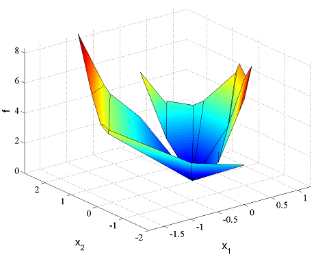
plot(domain(Jopt))

By using parametric solutions on uncertain max-plus models, various minimax schemes can easily be developed. See the [dynamic programming example] and [Examples RobustMPC robust MPC example] for details.