Nonconvex QP via piecewise affine models

To showcase the generality and convenience of interp1, let us answer a common question which addresses the problem of solving (possibly mixed-integer) quadratic programs using linear solvers, and to make matters worse, we study indefinite quadratic objectives.

Given indefinite structure

The simple idea we will use is to approximate the quadratic function as a piecewise affine function. Of course, this is not necessarily a good way to solve indefinite quadratic programs, but it is a common strategy (see this post for some alternatives). Let us assume we want to minimize the indefinite objective \(x^TQx - y^TRy\) with positive definite \(Q\) and \(R\) over the unit-box intersected with \(\sum x + \sum y = 1\).

n = 10;
x = sdpvar(n,1);
y = sdpvar(n,1);
Q = randn(n);Q = Q*Q';
R = randn(n);R = R*R';
Model = [-1 <= [x y] <= 1, sum(x) + sum(y) == 1];

To begin with, a problem here is that the model is multivariate, but interp1 only handles univariate data. To solve this, we factorize the quadratic functions and the objective into univariate functions \(\sum e_i^2 - \sum f_i^2\)

S = chol(Q);
T = chol(R);
e = sdpvar(n,1);
f = sdpvar(n,1);
Model = [-1 <= [x y] <= 1, sum(x) + sum(y) == 1, e == S*x, f == T*y];

Our next step is to introduce a piecewise affine approximation of every quadratic term \(e_i\) and \(f_i\) using interp1. To do this, we have to define the domain over which the functions are approximated, i.e., find lower and upper bounds on the elements in \(e\) and \(f\). We can conviently do that using boundingbox

[~,Le,Ue] = boundingbox(Model,[],e);
[~,Lf,Uf] = boundingbox(Model,[],f);

Generate a grid over the bounding boxes and define the piecewise affine approximators

N = 100;
E = repmat(Le,1,N) + repmat(linspace(0,1,N),n,1).*repmat(Ue-Le,1,N);
F = repmat(Lf,1,N) + repmat(linspace(0,1,N),n,1).*repmat(Uf-Lf,1,N);

f1 = interp1(E,E.^2,e,'lp');
f2 = interp1(F,F.^2,f,'lp');

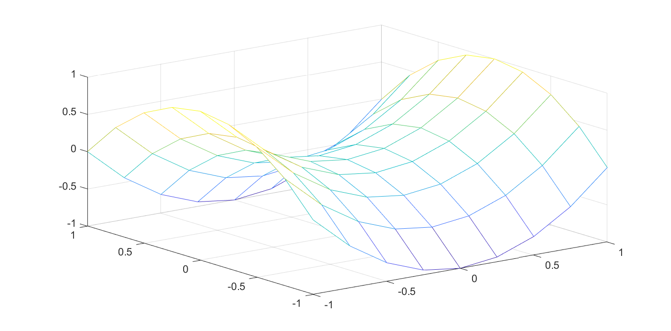
What we are doing here is essentially preparing for the following approximation (here in a more coarse sub-division to clearly see the affine structure)

z = -1:0.25:1;
mesh(z,z,z.^2-(z').^2)

With the flag ‘lp’, the way the interpolation is implemented depends on data and convexity propagation. An efficient linear programming based graph representation will be used if possible, while a mixed-integer sos2 approach is used otherwise. In our case, the first term is convex and will thus be implemented efficiently, while the second term requires sos2

optimize(Model,sum(f1)-sum(f2))

Partial convexity exploitation

If we have a convex mixed-integer quadratic programming solver and our goal only is to avoid the indefinite quadratic, there is no need to approximate the first convex part of the objective, so we can use a partially approximated model instead

Model = [-1 <= [x y] <= 1, sum(x) + sum(y) == 1, f == T*y];
optimize(Model,x'*Q*x-sum(f2))

Generic case

If we are given a general quadratic \(p(z)\) we can factorize it into a difference of convex quadratic functions by performing an eigenvalue factorization.

z = sdpvar(5,1);
p = (sum(z))^2 - sum(z.^2);
[H,c,b,z] = quaddecomp(p);
[V,D] = eig(full(H));
pos = find(diag(D)>0);
neg = find(diag(D)<0);
S = D(pos,pos)^.5*V(:,pos)';
T = (-D(neg,neg))^.5*V(:,neg)';

Note that \(S\) and \(T\) might have a different dimensions, meaning that \(e\) and \(f\) will have fewer elements than \(z\) (the number of elements in \(e\) will be equal to the number of positve eigenvalues in \(H\) and the number of elements in \(f\) will be equal to the number of negative eigenvalues in \(H\).

Applying this generic approach to our problem would be done by

n = 10;
x = sdpvar(n,1);
y = sdpvar(n,1);
Q = randn(n);Q = Q*Q';
R = randn(n);R = R*R';
p = x'*Q*x - y'*R*y;

% We don't know about the simple structure of p...
[H,c,b,z] = quaddecomp(p);
[V,D] = eig(full(H));
pos = find(diag(D)>0);
neg = find(diag(D)<0);
S = D(pos,pos)^.5*V(:,pos)';
T = (-D(neg,neg))^.5*V(:,neg)';

e = sdpvar(size(S,1),1);
f = sdpvar(size(T,1),1);
Model = [-1 <= [x y] <= 1, sum(x) + sum(y) == 1, e == S*z, f == T*z];
[~,Le,Ue] = boundingbox(Model,[],e);
[~,Lf,Uf] = boundingbox(Model,[],f);
N = 100;
E = repmat(Le,1,N) + repmat(linspace(0,1,N),n,1).*repmat(Ue-Le,1,N);
F = repmat(Lf,1,N) + repmat(linspace(0,1,N),n,1).*repmat(Uf-Lf,1,N);

f1 = interp1(E,E.^2,e,'lp');
f2 = interp1(F,F.^2,f,'lp');
optimize(Model,sum(f1)-sum(f2) + c'*z + b)

We can keep the convex part of course to see if the convex MIQP performs better than a full approximation via a MILP.

Model = [-1 <= [x y] <= 1, sum(x) + sum(y) == 1, f == T*z];
optimize(Model,z'*S'*S*z - sum(f2) + c'*z + b)

A drawback with the generic approach, compared to the more direct model above, is that some sparse block-structure is lost in the decompositions, which might lead to worse performance in the solver.