Nonconvex quadratic programming comparisons

The computational results reported below are a bit outdated. For more recent numbers and a more comparisons see the article Nonconvex quadratic programming and moments: 10 years later

A common question I get is along the lines how can I solve a nonconvex QP using SeDuMi?

The answer to the questions is a bit tricky, since it depends on what the user means with solve, and why SEDUMI is mentioned. Do you mean that you want to compute an exact solution and just assume that SEDUMI (or any SDP solver) can do this, or have you stumbled upon the notion of semidefinite relaxations and think semidefinite relaxations always solve the problem, or do you understand that a semidefinite relaxation only some times gives a solution, and primarily are used to compute lower bounds?

Some key-points

1. Nonconvex QPs can not be solved directly using SEDUMI.
2. Nonconvex QPs are NP-hard, and thus intractable (practically impossible to solve) in the general (non-trivially sized) case.
3. Semidefinite relaxations (and thus SEDUMI) can be used to compute lower bounds on the achievable objective.
4. Sometimes the semidefinite relaxation is tight and a solution can be recovered.
5. There are stronger semidefinite relaxations than the standard relaxation (based on the so called method of moments).
6. Adding redundant constraints can improve performance tremendously.
7. For a guaranteed solution, a global solver can be used as an (often better) alternative.

Semidefinite relaxations

To begin with, let us define a simple bound-constrained indefinite QP, and throw it at YALMIP.

Q = magic(5);
x = sdpvar(5,1);
optimize([-1 <= x <= 1],x'*Q*x)

If you have any nonlinear solver installed (such as FMINCON), YALMIP will call that solver. Some versions of CPLEX and QUADPROG also accept indefinite QPs, so it might happen that YALMIP calls any of these solvers. Note though, the solution is not guaranteed to be a globally optimal solution (CPLEX can compute globally optimal solutions by setting the ‘optimalitytarget’ option suitably)

Our first approach will be to manually pose the semidefinite relaxation of the indefinite QP. The first trick in semidefinite relaxations is to introduce a new matrix \(X\), intended to model \(xx^T\). We use the fact \(x^TQx=trace(QX)\) and conceptually pose the following problem

X = sdpvar(5);
optimize([-1 <= x <= 1, X == x*x'],trace(Q*X))

Of course, it makes no sense to try to solve this problem. Although the objective is linear, we have quadratically many variables, with a large number of quadratic equality constraints, a problem arguably far more complicated than the original problem.

The central step in a semidefinite relaxation is to replace the equality with an inequality, apply a Schur complement and append a rank constraint. We thus arrive at the following linear rank-constrained semidefinite problem (don’t even try to run the problem below, you do not have any solver installed to solve it)

X = sdpvar(5);
optimize([-1 <= x <= 1, [1 x';x X]>=0, rank([1 x';x X])==1],trace(Q*X))

Once again, we have arrived at an even harder problem. Rank-constrained semidefinite problems are extremely hard to solve, much harder than the original indefinite QP.

Hence, the final trick is to simply remove the rank constraint, and arrive at a linear semidefinite program, the first-order semidefinite relaxation.

X = sdpvar(5);
optimize([-1 <= x <= 1, [1 x';x X]>=0],trace(Q*X))

Now, three things can happen

1. The problem is unbounded from below. The semidefinite relaxation is thus useless and gives no information.
2. The problem is bounded and computes a lower bound. The semidefinite relaxation does however not give any solution since \(X\) does not equal \(xx’^T\).
3. The problem is bounded and computes a lower bound. In addition to this \(X\) equals \(xx’^T\), and the lower bound is thus tight and the computed value on \(x\) is a solution to the original problem.

For the particular problem we address here, the first-order relaxation is unbounded. Hence, it is useless and a stronger relaxation is required.

Stronger semidefinite relaxations

Stronger relaxations can be constructed manually fairly easily in YALMIP, but it is much easier to use ready-made software to perform this. One option is the separate package GloptiPoly. Another alternative is the sparsity exploiting semidefinite relaxation code SPARSEPOP which is interfaced in YALMIP. Here, we will use the built-in semidefinite relaxation module in YALMIP.

The simple semidefinite relaxation above, can be solved using the built-in semidefinite relaxation module using two different calls

sol = optimize([-1 <= x <= 1],x'*Q*x,sdpsettings('solver','moment'));
sol = solvemoment([-1 <= x <= 1],x'*Q*x);

Note that a switch from a local approach to a semidefinite relaxation thus can be done by simply telling YALMIP to use another solver.

With the call above, we solve exactly the same semidefinite relaxation as before, and the lower bound is of course still unbounded. In order to solve a stronger semidefinite relaxation, we tell the moment module to use a second-order relaxation.

ops = sdpsettings('solver','moment','moment.order',2)
sol = optimize([-1 <= x <= 1],x'*Q*x,ops)

You will now see that the lower bound is finite (roughly -83). However, YALMIP is not able to recover any solution. If YALMIP manages to extract a solution, it returns these (there may be many) through the field xoptimal in the output sol. The reason YALMIP fails to extract a solution, is that also the second-order relaxation also is too weak. For this problem, a third order relaxation is required.

ops = sdpsettings('solver','moment','moment.order',3)
sol = optimize([-1 <= x <= 1],x'*Q*x,ops)

YALMIP manages to extract two solutions, and we can check the objective value of these solutions, and compare with the lower bound

relaxvalue(x'*Q*x)
value(x'*Q*x)
assign(x,sol.xoptimal{1})
value(x'*Q*x)
assign(x,sol.xoptimal{2})
value(x'*Q*x)

Comparison with Global solver

Although semidefinite relaxations have had a huge impact on the field of nonconvex optimization, it must not be forgotten that standard global optimization often is competitive, at least when a solution is required and a lower bound not is sufficient. Switching to YALMIPs built-in global solver BMIBNB is trivial

ops = sdpsettings('solver','bmibnb')
sol = optimize([-1 <= x <= 1],x'*Q*x,ops)

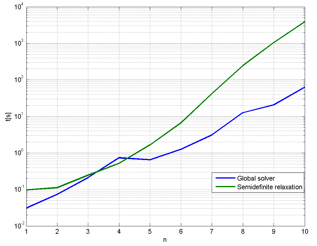
In contrast to what many people think, a global approach can be much more efficient than a semidefinite relaxation, if a tight solution is required. To illustrate this, let us solve our indefinite QP for growing dimensions (note that this code will take a long time to complete)

ops1 = sdpsettings('solver','bmibnb','bmibnb.maxiter',1000);
ops1 = sdpsettings(ops1,'bmibnb.uppersolver','fmincon');
ops2 = sdpsettings('solver','moment','moment.order',3)
for n = 1:10    
    Q = magic(n);
    x = sdpvar(n,1);
    sol = optimize([-1 <= x <= 1],x'*Q*x,ops1);
    comptimes(n,1) = sol.solvertime;
    sol = optimize([-1 <= x <= 1],x'*Q*x,ops2);
    comptimes(n,2) = sol.solvertime;
end
semilogy(1:10,comptimes)

As one can see in the figure below, the semidefinite relaxations are extremely slow to compute compared to a vanilla branch & bound solver, already for modest problem sizes (the semidefinite relaxations were solved using SEDUMI while the global solver used FMINCON and GUROBI)

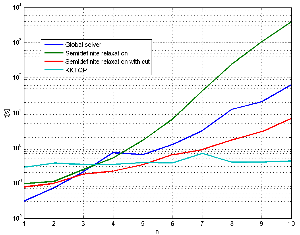
However, we can easily make semidefinite relaxations competitive here. Simply add redundant constraints on the squared variables, and the second-order relaxation turns out to be tight and a solution can be recovered in a couple of seconds for the case n = 10 (which takes almost an hour for the third-order relaxation)

ops2 = sdpsettings('solver','moment','moment.order',2);
sol = optimize([-1 <= x <= 1,x x.*x <= 1],x'*Q*x,ops2);

Still, we have alternative, possibly even faster, ways to solve the problem. By reformulating the nonconvex QP to a mixed-integer linear program, the problem can be solved in a fraction of a second. A KKT based indefinite QP solver is available in YALMIP (assuming you have an efficient MILP solver installed)

ops= sdpsettings('solver','kktqp');
sol = optimize([-1 <= x <= 1],x'*Q*x,ops);

We repeat the experiments above, now with the strengthened second-order relaxation, and the KKT based MILP approach. From the figure, it is clear the the last method is the most efficient for this problem family, and the solver used.

Suitable reading

[Lasserre 2001], Introduction to moment relaxations in YALMIP, Introduction to global optimization in YALMIP