Model predictive control - Explicit multi-parametric solution
YALMIP extends the parametric algorithms in MPT by adding a layer to enable binary variables and equality constraints. We can use this to find explicit solutions to, e.g., predictive control of PWA (piecewise affine) systems. Explicit solutions to MPC problems are solved using either one-shot approaches, or dynamic programming approaches.
One-shot with PWA model
Let us find the explicit solution to a variant of the MPC problem introduced in the hybrid MPC example. This will be a pretty advanced example, so let us start slowly by defining the some data.
yalmip('clear')
clear all
% Model data
A = [2 -1;1 0];
B1 = [1;0];  % Small gain for  x(1) > 0
B2 = [pi;0]; % Larger gain for x(1) < 0
C = [0.5 0.5];
nx = 2; % Number of states
nu = 1; % Number of inputs

% Prediction horizon
N = 4;
To simplify the code and the notation, we create state, control and region identifiers in cell arrays.
% States x(k), ..., x(k+N)
x = sdpvar(repmat(nx,1,N),repmat(1,1,N));
% Inputs u(k), ..., u(k+N) (last one not used)
u = sdpvar(repmat(nu,1,N),repmat(1,1,N));
% Binary for PWA selection
d = binvar(repmat(2,1,N),repmat(1,1,N));
We now run a loop to add constraints on all states and inputs. For the logic constraints to work well, it is extremely important that all variables are explicitly bounded. Read more about this in the logic programming) and the big-M tutorial. To prepare for the dynamic programming code later on, we setup the constraints back-wards in time.
constraints = [];
objective = 0;

for k = N-1:-1:1

    % Feasible region
    constraints = [constraints , -1 <= u{k}     <= 1,
                                 -1 <= C*x{k}   <= 1,
                                 -5 <= x{k}     <= 5,
                                 -1 <= C*x{k+1} <= 1,
                                 -5 <= x{k+1}   <= 5];
    % PWA Dynamics
    constraints = [constraints ,implies(d{k}(1),x{k+1} == A*x{k}+B1*u{k}),
                                implies(d{k}(2),x{k+1} == A*x{k}+B2*u{k});
                                implies(d{k}(1),x{k}(1) >= 0),
                                implies(d{k}(2),x{k}(1) <= 0)];

    % It is EXTREMELY important to add as many
    % constraints as possible to the binary variables
    constraints = [constraints, sum(d{k}) == 1];

    % Add stage cost to total cost
    objective = objective + norm(x{k},1) + norm(u{k},1);
end
The parametric variable here is the current state x{1}. In this optimization problem, there are many variables that we have no interest in x, d, and future u). To tell YALMIP that we only want the explicit optimizer for the current state u{1}, we use a fifth input argument.
[sol,diagn,Z,Valuefcn,Optimizer] = solvemp(constraints,objective ,[],x{1},u{1});
We plot the value function and the optimal solution
figure;plot(Valuefcn)
figure;plot(Optimizer)
To obtain the optimal control input for a specific state, we use value and assign as usual.
assign(x{1},[-1;1]);
value(Optimizer)
ans =
    0.9549
The optimal cost at this state is available in the value function
value(Valuefunction)
ans =
    4.2732
To convince our self that we have a correct parametric solution, let us compare it to the solution obtained by solving the problem for this specific state.
sol = optimize([constraints, x{1}==[-1;1],objective);
value(u{1})
ans =
    0.9549
value(obj)
ans =
    4.2732
Dynamic programming with LTI systems
The capabilities in YALMIP to work with piecewise functions and parametric programs enables easy coding of dynamic programming algorithms. The value function with respect to the parametric variable for a parametric linear program is a convex PWA function, and this is the function returned in the fourth output. YALMIP creates this function internally, and also saves information about convexity etc, and uses it as any other nonlinear operator (see more details below). For binary parametric linear programs, the value function is no longer convex, but a so called overlapping PWA function. This means that, at each point, it is defined as the minimum of a set of convex PWA function. This information is also handled transparently in YALMIP, it is simply another type of nonlinear operator. The main difference between the two function classes is that the second class requires introduction of binary variables when used.
Note, the algorithms described in the following sections are mainly intended for (piecewise) linear objectives. Dynamic programming with quadratic objective functions give rise to problems that are much harder to solve, although it is supported.
To illustrate how easy it is to work with these PWA functions, we will solve a predictive control using dynamic programming, instead of setting up the whole problem in one shot as we did above. As a first example, we solve a standard linear predictive control problem.
yalmip('clear')
clear all
% Model data
A = [2 -1;1 0];
B = [1;0];
C = [0.5 0.5];
nx = 2; % Number of states
nu = 1; % Number of inputs

% Prediction horizon
N = 4;
% States x(k), ..., x(k+N)
x = sdpvar(repmat(nx,1,N),repmat(1,1,N));
% Inputs u(k), ..., u(k+N) (last one not used)
u = sdpvar(repmat(nu,1,N),repmat(1,1,N));
Now, instead of setting up the problem for the whole prediction horizon, we only set it up for one step, solve the problem parametrically, take one step back, and perform a standard dynamic programming value iteration.
J{N} = 0;

for k = N-1:-1:1

    % Feasible region
    constraints = [-1 <= u{k}     <= 1,
                   -1 <= C*x{k}   <= 1,
                   -5 <= x{k}     <= 5,
                   -1 <= C*x{k+1} <= 1,
                   -5 <= x{k+1}   <= 5];

    % Dynamics
    constraints = [constraints, x{k+1} == A*x{k}+B*u{k}];

    % Cost in value iteration
    objective = norm(x{k},1) + norm(u{k},1) + J{k+1}

    % Solve one-step problem
    [sol{k},dgn{k},Uz{k},J{k},uopt{k}] = solvemp(constraints,objective,[],x{k},u{k});
end
Notice the minor changes needed compared to the one-shot solution. Important to understand is that the value function at step k will be a function in x{k}, hence when it is used at k-1, it will be a function penalizing the predicted state. Note that YALMIP automatically keeps track of convexity of the value function. Hence, for this example, no binary variables are introduced along the solution process.
To study the development of the value function, we can plot them.
for k = N-1:-1:1
 plot(J{k});hold on
end
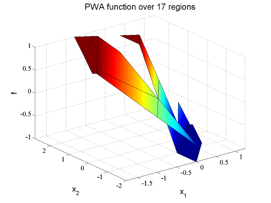
The final optimal control input can also be plotted.
clf;plot(uopt{1})
Of course, you can do the same thing by working directly with the numerical MPT data.
for k = N-1:-1:1
 mpt_plotPWA(sol{k}{1}.Pn,sol{k}{1}.Bi,sol{k}{1}.Ci);hold on
end
Why not solve the problem with a worst-peak cost! Notice the non-additive value iteration! Although this might look complicated using a mix of maximums, norms and piecewise value-functions , the formulation fits perfectly into the nonlinear operator framework in YALMIP. Additionally, we add a terminal-state weight by initializing the value function.
J{N} = norm(x{N},1);

for k = N-1:-1:1

    % Feasible region
     constraints = [-1 <= u{k}     <= 1,
                    -1 <= C*x{k}   <= 1,
                    -5 <= x{k}     <= 5,
                    -1 <= C*x{k+1} <= 1,
                    -5 <= x{k+1}   <= 5];
    % Dynamics
     constraints = [constraints, x{k+1} == A*x{k}+B*u{k}];

    % Cost in value iteration
    objective = max(norm([x{k};u{k}],inf),J{k+1})

    % Solve one-step problem
    [sol{k},dgn{k},Uz{k},J{k},uopt{k}] = solvemp(constraints,objective,[],x{k},u{k});
end
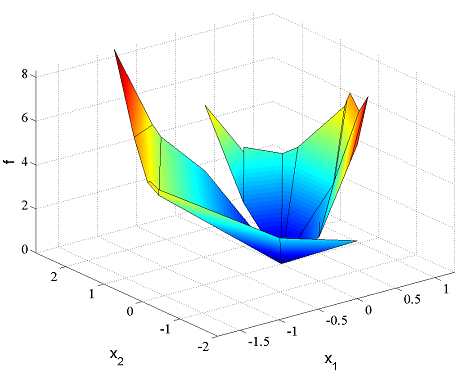
Dynamic programming with PWA systems
As mentioned above, the difference between the value function from a parametric LP and a parametric LP with binary variables is that convexity of the value function no longer is guaranteed. In practice, this means that (additional) binary variables are required when the the value function is used in an optimization problem. This is done automatically in YALMIP through the [nonlinear operator framework], but it is extremely important to realize that the value function from a binary problem is much more complex than the one resulting from a standard parametric problem. Nevertheless, working with the objects is easy, as the following example illustrates. In this case, we solve the dynamic programming problem for our PWA system
yalmip('clear')
clear all
% Model data
A = [2 -1;1 0];
B1 = [1;0];
B2 = [pi;0]; % Larger gain for negative first state
C = [0.5 0.5];
nx = 2; % Number of states
nu = 1; % Number of inputs

% Prediction horizon
N = 4;
% States x(k), ..., x(k+N)
x = sdpvar(repmat(nx,1,N),repmat(1,1,N));
% Inputs u(k), ..., u(k+N) (last one not used)
u = sdpvar(repmat(nu,1,N),repmat(1,1,N));
% Binary for PWA selection
d = binvar(repmat(2,1,N),repmat(1,1,N));
Just as in the LTI case, we set up the problem for the one step case, and use the value function from the previous iteration.
J{N} = 0;

for k = N-1:-1:1

    % Feasible region
    constraints = [-1  <= u{k}     <= 1,
                    -1 <= C*x{k}   <= 1,
                    -5 <= x{k}     <= 5,
                    -1 <= C*x{k+1} <= 1,
                    -5 <= x{k+1}   <= 5];
    % PWA Dynamics
    constraints = [constraints, implies(d{k}(1),x{k+1} == A*x{k}+B1*u{k}),
                                implies(d{k}(2),x{k+1} == A*x{k}+B2*u{k}),
                                implies(d{k}(1),x{k}(1) >= 0),
                                implies(d{k}(2),x{k}(1) <= 0),
                                sum(d{k}) == 1];

    % Cost in value iteration
    objective = norm(x{k},1) + norm(u{k},1) + J{k+1}

    % Solve one-step problem
    [sol{k},dgn{k},Uz{k},J{k},uopt{k}]=solvemp(constraints,objective,[],x{k},u{k});
end
Dynamic programming with polytopic systems
As a final example, let us compute a robust MPC solution to an uncertain system. We now assume that the switch between the two input gains B1 and B2 is unknown. To address this, a worst-case (minimax) solution will be computed. Although there is built-in support for uncertain data and robust optimization via the [robust optimization framework], we will have to model this manually. To solve the worst-case problem, we first need robust feasibility, i.e. the one step prediction in the DP iteration should be robustly feasible. Secondly, instead of minimizing the stage-cost plus the cost-to-go, we have to minimize the stage-cost plus the worst-case cost-to-go.
In the DP code above, we have connected the current state, the next state and the value function (which is a function of the next state) via equality constraints between x{k} and x{k+1}, or via implications. This cannot be done here, since the equality would involve uncertainty. Instead, we explicitly construct a value function for all extreme uncertainties (remember, this problem is convex, so we only need to check the extreme cases) and minimize the maximum of these. The trick to do this in YALMIP is to use the [replace]] command. Having this command, the rest of the code is straightforward.
yalmip('clear')
clear all
% Model data
A = [2 -1;1 0];
B1 = [1;0];
B2 = [pi;0]; % Larger gain for negative first state
C = [0.5 0.5];
nx = 2; % Number of states
nu = 1; % Number of inputs

% Prediction horizon
N = 4;
% States x(k), ..., x(k+N)
x = sdpvar(repmat(nx,1,N),repmat(1,1,N));
% Inputs u(k), ..., u(k+N) (last one not used)
u = sdpvar(repmat(nu,1,N),repmat(1,1,N));
% Binary for PWA selection
d = binvar(repmat(2,1,N),repmat(1,1,N));

J{N} = 0;

for k = N-1:-1:1

    % Feasible region
    constraints = [-1 <= u{k}     <= 1,
                   -1 <= C*x{k}   <= 1,
                   -5 <= x{k}     <= 5];

    % Robustly feasible predictions
    constraints = [-1 <= C*(A*x{k}+B1*u{k}) <= 1,
                   -5 <= A*x{k}+B1*u{k}     <= 5,
                   -1 <= C*(A*x{k}+B2*u{k}) <= 1,
                   -5 <= A*x{k}+B2*u{k}     <= 5];

    % Extreme predictions
    J1 = replace(J{k+1},x{k+1},A*x{k}+B1*u{k});
    J2 = replace(J{k+1},x{k+1},A*x{k}+B2*u{k});

    % worst-case cost in value iteration
    objective = norm(x{k},1) + norm(u{k},1) + max(J1,J2);

    % Solve one-step problem
    [sol{k},dgn{k},Uz{k},J{k},uopt{k}] = solvemp(constraints ,objective ,[],x{k},u{k});
end
Note that quadratic objective functions not can be used for dynamic programming with polytopic systems in YALMIP. The reason is that the max operator applied to quadratic functions will generate quadratic constraints, which not is supported by the parametric solvers in MPT .
Behind the scenes and advanced use
The first thing that might be a bit unusual to the advanced user is the piecewise functions that YALMIP returns in the fourth and fifth output from solvemp. In principle, they are specialized [pwf] objects. To create a PWA value function after solving a multi-parametric LP, the following command is used.
Valuefunction = pwf(sol,x,'convex')
The pwf command will recognize the MPT solution structure and create a PWA function based on the fields Pn, Bi and Ci. The dedicated [nonlinear operator] is implemented in the file pwa_yalmip.m . The [nonlinear operator] will exploit the fact that the PWA function is convex and implement an efficient epi-graph representation. In case the PWA function is used in a nonconvex fashion (i.e. YALMIPs automatic convexity propagation fails), a MILP implementation is also available.
If the field Ai is non-empty (solution obtained from a multi-parametric QP), a corresponding PWQ function is created (pwq_yalmip.m).
To create a PWA function representing the optimizer, two things have to be changed. To begin with, YALMIP searches for the Bi and Ci fields, but since we want to create a PWA function based on Fi and Gi fields, the field names have to be changed. Secondly, the piecewise optimizer is typically not convex, so a general PWA function is created instead (requiring 1 binary variable per region if the variable later actually is used in an optimization problem.)
sol.Ai = cell(1,length(sol.Ai));
sol.Bi = sol.Fi;
sol.Ci = sol.Gi;
Optimizer = pwf(sol,x,'general')
A third important case is when the solution structure returned from solvemp is a cell with several MPT structures. This means that a multiparametric problem with binary variables was solved, and the different cells represent overlapping solutions. One way to get rid of the overlapping solutions is to use the MPT command mpt_removeOverlaps.m and create a PWA function based on the result. Since the resulting PWA function typically is nonconvex, we must create a general function.
sol_single = mpt_removeOverlaps(sol);
Valuefunction = pwf(sol_single,x,'general')
This is only recommended if you just intend to plot or investigate the value function. Typically, if you want to continue computing with the result, i.e. use it in another optimization problem, as in the dynamic programming examples above, it is recommended to keep the overlapping solutions. To model a general PWA function, 1 binary variable per region is needed. However, by using a dedicated nonlinear operator for overlapping convex PWA functions, only one binary per PWA function is needed.
Valuefunction = pwf(sol,x,'overlapping')
As we have seen in the examples above, the PWA and PWQ functions can be plotted. This is currently nothing but a simple hack. Normally, when you apply the [plot] command to an sdpvar object, the corresponding double values are plotted. However, if the input is a simple scalar PWA or PWQ variable, the underlying MPT structures will be extracted and the plot commands in MPT will be called.
