Model predictive control - Basics

To prepare for the hybrid, explicit and robust MPC examples, we solve some standard MPC examples. As we will see, MPC problems can be formulated in various ways in YALMIP.

To begin with, let us define the numerical data that defines our LTI system and the control problem.

yalmip('clear')
clear all

% Model data
A = [2 -1;1 0.2];
B = [1;0];
nx = 2; % Number of states
nu = 1; % Number of inputs

% MPC data
Q = eye(2);
R = 2;
N = 7;

% Initial state
x0 = [3;1];

Our optimization problem is to minimize a finite horizon cost of the state and control trajectory, while satisfying constraints.

Explicit prediction form

The first version we implement (we will propose an often better approaches below) explicitly expresses the predicted states as a function of a given current state and the future control sequence. We simply loop the simulation equations and gather constraints and objective terms along the horizon. Notice the quick definition of a list of control inputs.

u = sdpvar(repmat(nu,1,N),repmat(1,1,N));

constraints = [];
objective = 0;
x = x0;
for k = 1:N
 x = A*x + B*u{k};
 objective = objective + norm(Q*x,1) + norm(R*u{k},1);
 constraints = [constraints, -1 <= u{k}<= 1, -5<=x<=5];
end

Once the constraints and objective function have been generated, we can solve the optimization problem (in this case, a linear programming problem in the decision variable u and variables required to model the norms).

optimize(constraints,objective);
value(u{1})

Setting up a problem like this every time we have a new initial state is a waste of computational effort. Almost all CPU time will be spent in YALMIPs overhead to define the model and convert the model to solver specific format, and not in the actual solution of the optimization problem.

To avoid some of the over-head, we formulate the problem with the initial state as a decision variable.

u = sdpvar(repmat(nu,1,N),repmat(1,1,N));
x0 = sdpvar(2,1);

constraints = [];
objective = 0;
x = x0;
for k = 1:N
 x = A*x + B*u{k};
 objective = objective + norm(Q*x,1) + norm(R*u{k},1);
 constraints = [constraints, -1 <= u{k}<= 1, -5<=x<=5];
end

We can now obtain a solution from an arbitrary initial state, by simply constraining the initial state. The benefit now is that we do not have to redefine the complete model everytime the initial state changes, but simply make a small addition to it. The overhead in YALMIP to convert to solver specific format remains though. Of course, the drawback is that there are some extra variables and constraints, but the computational impact of this is absolutely minor.

optimize([constraints, x0 == [3;1]],objective);
value(u{1})

Improving simulation performance

A large amount of time is still spent in optimize to convert from the YALMIP model to the numerical format used by the solver. If we want to, e.g., simulate the closed-loop system, this is problematic. To avoid this, we compile the numerical model once by using the optimizer command. For illustrative purposes, we allow the solver to print its output. Normally, this would be turned of when using optimizer (once we know everything works, never turn off display until everything works as expected)

ops = sdpsettings('verbose',2);
controller = optimizer(constraints,objective,ops,x0,u{1});

We can now simulate the system using very simple code (notice that an optimization problem still is solved every time the controller object is referenced, but most of YALMIPs overhead is avoided)

x = [3;1]
for i = 1:5
 uk = controller{x}
 x = A*x + B*uk
end

Of course, we can extract additional variables from the solution by requesting these. Here, we output the whole predicted control sequence and iteratively plot this

ops = sdpsettings('verbose',2);
controller = optimizer(constraints,objective,ops,x0,[u{:}]);
x = [3;1];
clf;
hold on
for i = 1:15
  U = controller{x};
  stairs(i:i+length(U)-1,U,'r')
  x = A*x + B*U(1);
  pause(0.05)
  stairs(i:i+length(U)-1,U,'k')
end

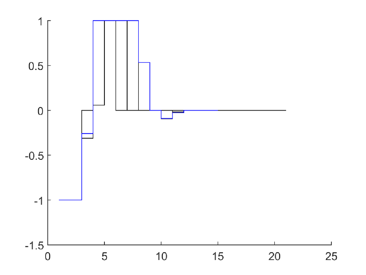
Implicit prediction form

The optimization problem generated by the formulation above is a problem in the control variables (and the initial state). This is typically the approach used in standard introductory texts on MPC. However, in many cases, it is both convenient and more numerically sound to optimize over both the control input and the state predictions, and model the system dynamics using equality constraints instead of assignments. Although this yields a larger optimization problem, it has a lot of structure and sparsity, which typically is very well exploited by the solver.

An implicit form is easily coded in YALMIP with minor changes to the code above. We skip the options now as we do not need the print-out any longer

u = sdpvar(repmat(nu,1,N),repmat(1,1,N));
x = sdpvar(repmat(nx,1,N+1),repmat(1,1,N+1));

constraints = [];
objective = 0;
for k = 1:N
 objective = objective + norm(Q*x{k},1) + norm(R*u{k},1);
 constraints = [constraints, x{k+1} == A*x{k} + B*u{k}];
 constraints = [constraints, -1 <= u{k}<= 1, -5<=x{k+1}<=5];
end

controller = optimizer(constraints, objective,[],x{1},[u{:}]);

x = [3;1];
clf;
hold on
implementedU = [];
for i = 1:15
  U = controller{x};  
  stairs(i:i+length(U)-1,U,'r')
  x = A*x + B*U(1);
  pause(0.05)
  stairs(i:i+length(U)-1,U,'k')
  implementedU = [implementedU;U(1)];
end
stairs(implementedU,'b')

The models are easily extended to more complicated scenarios. Here we simulate the case with a reference trajectory preview, and a known, assumed constant, disturbance. We also want to plot the optimal predicted output with the reference. Inputs are not allowed to make changes larger than 0.15 and we switch to a quadratic objective function. To make matters worse, we do not know the value of the B matrix at compile time, as it can change. Hence, we make it a parameter. Since we now have a nonlinear parameterization, we explicitly select a QP solver, to communicate to YALMIP that we know the problem will be a convex QP for fixed value of the parameters (the bilinearities between B and u will turn linear once B is fixed)

yalmip('clear')
clear all

% Model data
A = [2 -1;1 0.2];
B = sdpvar(2,1);
E = [1;1];
nx = 2; % Number of states
nu = 1; % Number of inputs

% MPC data
Q = eye(2);
R = 2;
N = 20;


ny = 1;
C = [1 0];

u = sdpvar(repmat(nu,1,N),repmat(1,1,N));
x = sdpvar(repmat(nx,1,N+1),repmat(1,1,N+1));
r = sdpvar(repmat(ny,1,N+1),repmat(1,1,N+1));
d = sdpvar(1);
pastu = sdpvar(1);

constraints = [-.1 <= diff([pastu u{:}]) <= .1];
objective = 0;
for k = 1:N
    objective = objective + (C*x{k}-r{k})'*(C*x{k}-r{k}) + u{k}'*u{k};
    constraints = [constraints, x{k+1} == A*x{k}+B*u{k}+E*d];
    constraints = [constraints, -1 <= u{k}<= 1, -5<=x{k+1}<=5];
end
objective = objective + (C*x{N+1}-r{N+1})'*(C*x{N+1}-r{N+1});

parameters_in = {x{1},[r{:}],d,pastu,B};
solutions_out = {[u{:}], [x{:}]};

controller = optimizer(constraints, objective,sdpsettings('solver','gurobi'),parameters_in,solutions_out);
x = [0;0];
clf;
disturbance = randn(1)*.01;
oldu = 0;
hold on
xhist = x;
for i = 1:300
    if i < 50
        Bmodel = [1;0];
    else
        Bmodel = [.9;.1];
    end
    future_r = 3*sin((i:i+N)/40);    
    inputs = {x,future_r,disturbance,oldu,Bmodel};
    [solutions,diagnostics] = controller{inputs};    
    U = solutions{1};oldu = U(1);
    X = solutions{2};
    if diagnostics == 1
        error('The problem is infeasible');
    end    
    subplot(1,2,1);stairs(i:i+length(U)-1,U,'r')
    subplot(1,2,2);cla;stairs(i:i+N,X(1,:),'b');hold on;stairs(i:i+N,future_r(1,:),'k')
    stairs(1:i,xhist(1,:),'g')    
    x = A*x + Bmodel*U(1)+E*disturbance;
    xhist = [xhist x];
    pause(0.05)   
    % The measured disturbance actually isn't constant, it changes slowly
    disturbance = 0.99*disturbance + 0.01*randn(1);
end