Model predictive control - robust solutions
This example illustrates an application of the [robust optimization framework].
Robust optimization is a natural tool for robust control, i.e., derivation of control laws such that constraints are satisfied despite uncertainties in the system, and/or worst-case performance objectives. Various formulations for robust MPC were introduced in Löfberg 2003, and we will use YALMIPs robust optimization framework to derive some of the robustified optimization problems automatically. The example will essentially solve various versions of Example (7.4) in Löfberg 2003.
The system description is \(x_{k+1} = Ax_k + Bu_k+Ew_k, y_k = Cx_k\)
A = [2.938 -0.7345 0.25;4 0 0;0 1 0];
B = [0.25;0;0];
C = [-0.2072 0.04141 0.07256];
E = [0.0625;0;0];
Open-loop minimax solution
A prediction horizon N=10 is used. We first derive a symbolic expression of the future outputs by symbolically simulating the predictions. Note that we use an explicit representation of the predictions. In the explicit MPC example, we used an implicit representation by declaring the state updates via equality constraints. This does not make sense here, since we want the model to hold robustly. An uncertain equality constraint does not make sense. Instead, we explicitly express future states as a function of the current state, and the control and disturbance sequence.
N = 10;
U = sdpvar(N,1);
W = sdpvar(N,1);
x = sdpvar(3,1);

Y = [];
xk = x;
for k = 1:N
 xk = A*xk + B*U(k)+E*W(k);
 Y = [Y;C*xk];
end
The input is bounded, and the objective is to stay as close as possible to the level \(y=1\) while guaranteeing that \(y \leq 1\) is satisfied despite the disturbances \(w\).
F = [Y <= 1, -1 <= U <= 1];
objective = norm(Y-1,1) + norm(U,1)*0.01;
The uncertainty is known to be bounded.
G = [-1 <= W <= 1]
To speed up the simulations (the code is still pretty slow), the robustfied model is derived once without solving it using robustmodel
[Frobust,h] = robustify(F + G,objective,[],W);
The derived model can now be used a standard YALMIP model, allowing us to simulate the closed-loop system by repeatedly solving the problem.
xk = [0;0;0];
ops = sdpsettings;
for i = 1:25
optimize([Frobust, x == xk(:,end)],h,ops);
xk = [xk A*xk(:,end) + B*value(U(1)) + E*(-1+2*rand(1))];
end
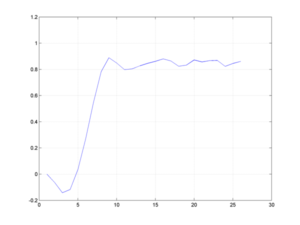
plot(C*xk)
To speed up the simulation further, we can use the optimizer construction. It is applicable here since the changing part of the optimization problem is the current state, which enters affinely in the model.
controller = optimizer([F, G, uncertain(W)],objective,ops,x,U(1));
xk = [0;0;0];
for i = 1:25
    xk = [xk A*xk(:,end) + B*controller{xk(:,end)} + E*(-1+2*rand(1))];
end
plot(C*xk)
Indeed, the solution satisfies the hard constraint, but the steady-state level on \(y\) is far away from the desired level. The reason is the open-loop assumption in the problem. The input sequence computed at time \(k\) has to take all future disturbances into account, and does not use the fact that MPC is implemented in a receding horizon fashion.
A better solution is a closed-loop assumption that exploits the fact that future inputs effectively are functions of future states (we will solve MPC problems in the future over new prediction horizons with measured states). This gives a lot less conservative solution, but the solution is, if not unsolvable, very hard. Typical solution require dynamic programming strategies, or brute-force enumeration. A tractable alternative was introduced in Löfberg 2003.
Approximate closed-loop minimax solution
The idea in Löfberg 2003 was to parameterize future inputs as affine functions of past disturbances. This, in contrast to parameterization in past states, lead to convex and tractable problems.
We create a causal feedback \(U = LW + V\) and derive the predicted states.
V = sdpvar(N,1);
L = sdpvar(N,N,'full').*(tril(ones(N))-eye(N));

U = L*W + V;

Y = [];
xk = x;
for k = 1:N
 xk = A*xk + B*U(k)+E*W(k);
 Y = [Y;C*xk];
end
A reasonable implementation of the worst-case scenario with this approximate closed-loop feedback is given by the following code.
F = [Y <= 1, -1 <= U <= 1];
objective = norm(Y-1,1) + norm(U,1)*0.01;

[Frobust,h] = robustify([F, G],objective,[],W);

xk = [0;0;0];
ops = sdpsettings;
for i = 1:25
    optimize([Frobust, x == xk(:,end)],h,ops);
    xk = [xk A*xk(:,end) + B*value(U(1)) + E*(-1+2*rand(1))];
end

hold on
plot(C*xk,'r')
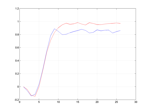
Obviously, the performance is far better (although we admittedly used different disturbance realizations, but the results are consistent if you run the simulations repeatedly).
Multiparametric solution of approximate closed-loop minimax problem
The robust optimization framework is integrated in the over-all infrastructure in YALMIP. Hence, a model can be robustified, and then sent to the multiparametric solver MPT in order to get a multi-parametric solution.
In our case, we want to have a multi-parametric solution with respect to the state \(x_k\). One way to compute the parametric solution is to first derive the robustified model, and send this to the parametric solver.
[Frobust,h] = robustify(F + G,objective,[],W);
sol = solvemp(Frobust,h,[],x);
Alternatively, we can send the uncertain model directly to solvemp, but we then have to declare the uncertain variables via the command uncertain
sol = solvemp([F,G,uncertain(W)],objective,[],x);
Dynamic programming solution to closed-loop minimax problem
It should be mentioned that, for some problems, an exact closed-loop solution can probably be computed more efficiently with dynamic programming along the lines of dynamic programming version of explicit mpc
Recall the DP code for the dynamic programming example for LTI systems to solve our problem without any uncertainty.
% Model data
A = [2.938 -0.7345 0.25;4 0 0;0 1 0];
B = [0.25;0;0];
C = [-0.2072 0.04141 0.07256];
E = [0.0625;0;0];
nx = 3; % Number of states
nu = 1; % Number of inputs

% Prediction horizon
N = 10;
% States x(k), ..., x(k+N)
x = sdpvar(repmat(nx,1,N),repmat(1,1,N));
% Inputs u(k), ..., u(k+N) (last one not used)
u = sdpvar(repmat(nu,1,N),repmat(1,1,N));

J{N} = 0;

for k = N-1:-1:1

    % Feasible region
    F = [-1 <= u{k} <= 1, C*x{k} <= 1, C*x{k+1} <= 1];

    % Bounded exploration space
    % (recommended for numerical reasons)
    F = [F, -100 <= x{k} <= 100];

    % Dynamics
    F = [F, x{k+1} == A*x{k}+B*u{k}];

    % Cost in value iteration
    obj = norm(C*x{k}-1,1) + norm(u{k},1)*0.01 + J{k+1};

    % Solve one-step problem
    [sol{k},diagnost{k},Uz{k},J{k},Optimizer{k}] = solvemp(F,obj,[],x{k},u{k});
end
We will now make some small additions to solve this problem robustly, i.e., minimize worst-case cost and satisfy constraints for all disturbances.
The first change is that we cannot work with equality constraints to define the state dynamics, since the dynamics are uncertain. Instead, we add constraints on the uncertain prediction equations.
Furthermore, the value function J{k+1} is defined in terms of the variable x{k+1}, but since we do not link x{k+1} with x{k} and u{k} with an equality constraint because of the uncertainty, we need to redefine the value function in terms of the uncertain prediction, to make sure that the objective function will be the worst-case cost.
% Uncertainty w(k), ..., w(k+N) (last one not used)
w = sdpvar(repmat(1,1,N),repmat(1,1,N));

J{N} = 0;

for k = N-1:-1:1

    % Feasible region
    F = [-1 <= u{k}     <= 1, C*x{k} <= 1];
    F = [F, C*(A*x{k} + B*u{k} + E*w{k}) <= 1];

    % Bounded exploration space
    F = [F, -100 <= x{k} <= 100];

    % Uncertain value function
    Jw = replace(J{k+1},x{k+1},A*x{k} + B*u{k} + E*w{k});

    % Declare uncertainty model
    F = [F, uncertain(w{k})];
    F = [F, -1 <= w{k} <= 1];

    % Cost in value iteration
    obj = norm(C*x{k}-1,1) + norm(u{k},1)*0.01 + Jw;

    % Solve one-step problem
    [sol{k},diagnost{k},Uz{k},J{k},Optimizer{k}] = solvemp(F,obj,[],x{k},u{k});
end
Note that this multiparametric problem seems to grow large, hence it will take a fair amount of time to compute it. Rest assured though, we are constantly working on improving performance in both MPT and YALMIP.
