Pre- and post-processing sum-of-squares programs
This example accompanies the paper Löfberg 2009.
Sum-of-squares has recently become a fairly well-established technique to attack problems involving polynomial constraints and objective functions Parrilo 2003. However, although sum-of-squares converts the original, theoretically intractable, polynomial problem to an SDP which can be solved using convex optimization, the problems that are generated are often huge, and numerically ill-conditioned.
In this example, we will take a look at features in YALMIP to address these issues.
Pre-processing
Sum-of-squares problems grow large very fast, so structure exploitation is needed for anything but small academic examples. YALMIP implements a couple of strategies to do this. Let us solve a simple problem where we first turn off all pre-processing.
x = sdpvar(1,1);
y = sdpvar(1,1);
z = sdpvar(1,1);
p = 12+y^2-2*x^3*y+2*y*z^2+x^6-2*x^3*z^2+z^4+x^2*y^2;

options = sdpsettings('sos.newton',0,'sos.congruence',0);
[sol,v,Q] = solvesos(sos(p),[],options);
-------------------------------------------------------------------------
YALMIP SOS module started...
-------------------------------------------------------------------------
Detected 0 parametric variables and 3 independent variables.
Detected 0 linear inequalities, 0 equality constraints and 0 LMIs.
Using kernel representation (options.sos.model=1).
Initially 15 monomials in R^3
The output reveals that YALMIP uses 15 monomials in the decomposition of the polynomial, hence the SDP will have a size 15x15. However, if you display the Gramian solution Q{1} after solving the problem, you will notice that it contains mainly zeros. This indicates that many of the monomials in the basis are not used.
Newton polytope
Indeed, if we turn on the Newton polytope pre-processing (which is on by default), the number of monomials are reduced to 9.
options = sdpsettings('sos.newton',1,'sos.congruence',0);
[sol,v,Q] = solvesos(sos(p),[],options);
-------------------------------------------------------------------------
YALMIP SOS module started...
-------------------------------------------------------------------------
Detected 0 parametric variables and 3 independent variables.
Detected 0 linear inequalities, 0 equality constraints and 0 LMIs.
Using kernel representation (options.sos.model=1).
Initially 15 monomials in R^3
Newton polytope (5 LPs).........Keeping 9 monomials (0.078125sec)
A smaller problem is now solved, but if you display the solution Q{1}, you will see that there is still a significant amount of zeros in the Gramian, indicating that more can be done.
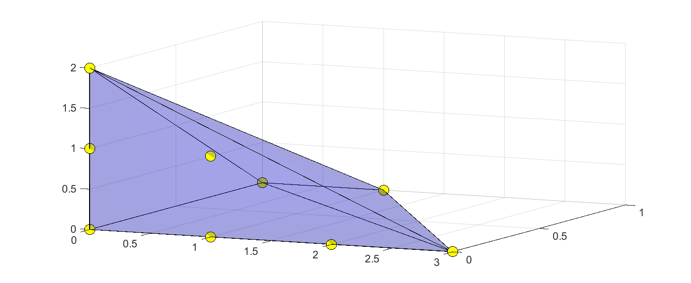
The Newton polytope vertices can be extracted with some use of internal utility functions and then used to define a polytope to plot.
clf
N = getexponentbase(newtonmonoms(p),[x y z]);
s = sdpvar(length(N),1);q = sdpvar(3,1);
plot([q == N'*s, sum(s)==1,s>=0],q,'b',[],sdpsettings('plot.shade',0.2))
hold on
m = plot3(N(:,1),N(:,2),N(:,3),'yo');
set(m,'Markersize',10);
set(m,'Markerface','yellow');
Symmetry reduction
By turning on the congruence feature, YALMIP will search for simple symmetries in the polynomial, and quickly block-diagonalize the problem. This can save a lot of computational effort, and more importantly, leads to much better conditioned SDP problems.
options = sdpsettings('sos.newton',1,'sos.congruence',1);
[sol,v,Q] = solvesos(sos(p),[],options);
-------------------------------------------------------------------------
YALMIP SOS module started...
-------------------------------------------------------------------------
Detected 0 parametric variables and 3 independent variables.
Detected 0 linear inequalities, 0 equality constraints and 0 LMIs.
Using kernel representation (options.sos.model=1).
Initially 15 monomials in R^3
Newton polytope (5 LPs).........Keeping 9 monomials (0.078125sec)
Finding symmetries..............Found 1 symmetry  (0sec)
Partitioning using symmetry.....2x2(1) 7x7(1)
YALMIP finds a symmetry to exploit and decomposes the Gramian to two smaller blocks. However, if you look at the solution Q{1}, you will note that there are still a vast amount of zeros and structure, indicating that there is more to be done. The pre-processing can not find this though. Instead, we turn to post-postprocessing.
Post-processing
The strongest feature in the post-processing code in YALMIP is the capability to analyze a solution, propose an improved block-diagonalization based on this, and resolve the problem. This can reduce the size of the decomposition significantly, and lead to much improved numerical conditioning.
This a-posteriori block-diagonalization is turned off by default. To turn it on, we have to change the option sos.numblkdg to a non-zero number. This number controls a threshold in the algorithm, basically controlling when a number can be considered to be zero. We solve the problem above again, and let YALMIP search for an improved block structure.
options = sdpsettings('sos.numblkdg',1e-4);
[sol,v,Q] = solvesos(sos(p),[],options);
You will see that the SDP solver is called three times, indicating that YALMIP actually finds some interesting structure in the numerical solutions. Indeed, displaying Q{1} reveals that the final decomposition only uses 5 monomials, and has a nice block-diagonal structure.
 Q{1}

ans =

   12.0000         0         0         0         0
         0    1.0000   -1.0000    1.0000         0
         0   -1.0000    1.0000   -1.0000         0
         0    1.0000   -1.0000    1.0000         0
         0         0         0         0    1.0000
As a more impressive example, consider the following polynomial, studied in Parrilo and Peretz 2004
x = sdpvar(1,1);
y = sdpvar(1,1);
z = sdpvar(1,1);
w = sdpvar(1,1);
p = 8*x^6*w^6*y^2+4*z^4*y^8*x^2+4*z^4*y^4*x^4+8*z^4*y^6*x^2+...
4*x^8*w^6*y^2+4*z^4*y^4*x^2+4*z^6*y^8*x^2+8*y^2*x^6*w^4+...
4*x^4*y^4*w^4-2*x^6*y^6-16*z^4*y^4*x^4*w^2-16*z^4*y^4*x^2*w^4-...
20*z^4*y^4*x^6*w^2-24*z^4*y^4*x^6*w^4+12*z^4*y^6*x^2*w^2-...
8*z^4*y^6*x^2*w^4+4*z^4*y^6*x^4*w^2-24*z^4*y^6*x^4*w^4-...
16*z^4*y^6*x^6*w^2-40*z^4*y^4*x^4*w^4-4*z^4*y^2*x^2*w^2-...
8*z^4*y^2*x^2*w^4-12*z^4*y^2*x^4*w^2-16*z^4*y^2*x^4*w^4-...
12*z^4*y^2*x^6*w^2-8*z^4*y^2*x^6*w^4-4*z^4*y^2*x^8*w^2-...
16*z^4*y^6*x^6*w^4+8*z^4*y^8*x^2*w^2+12*z^4*y^8*x^4*w^2-...
6*y^2*x^6*z^2*w^2-2*y^2*x^8*z^2*w^2-14*x^4*y^4*z^2*w^2-...
6*x^2*y^4*z^2*w^2-6*x^4*y^2*z^2*w^2-6*x^2*y^6*z^2*w^2-...
10*x^4*y^6*z^2*w^2-10*y^4*x^6*z^2*w^2-2*x^2*y^8*z^2*w^2-...
20*x^6*y^6*z^2*w^2+6*y^4*x^8*z^2*w^2+6*x^4*y^8*z^2*w^2+...
12*z^2*w^4*y^2*x^6-12*z^2*w^4*x^2*y^4-16*z^2*w^4*x^4*y^4+...
4*z^2*w^4*x^6*y^4-12*z^2*w^4*x^2*y^6-20*z^2*w^4*x^4*y^6+...
8*z^2*w^4*x^8*y^2+4*x^4*y^2*w^4+x^4*w^4+2*x^6*w^4+x^8*w^4+...
z^4*y^4+2*z^4*y^6+z^4*y^8+x^8*y^4+x^4*y^8+8*x^6*y^4*w^4+4*x^8*y^2*w^4+...
8*z^4*y^6*x^4+6*z^4*y^8*x^4-4*z^4*y^6*x^6+2*z^4*y^4*x^8+...
3*z^4*y^4*w^2+2*z^4*y^4*w^4+6*z^4*y^6*w^2+4*z^4*y^6*w^4+...
3*z^4*y^8*w^2+2*z^4*y^8*w^4-6*x^6*y^6*z^2+3*y^4*x^8*z^2+...
3*x^4*y^8*z^2-6*x^6*y^6*w^2+3*x^8*y^4*w^2+3*x^4*y^8*w^2+...
3*z^2*w^4*x^4+6*z^2*w^4*x^6+3*z^2*w^4*x^8+2*z^4*w^4*x^4+...
4*z^4*w^4*x^6+2*z^4*w^4*x^8-16*z^2*w^4*x^6*y^6-4*z^2*w^4*x^2*y^8+...
12*z^2*w^4*x^8*y^4-4*x^2*w^4*y^2*z^2-2*x^2*y^2*z^2*w^2+...
8*x^8*y^4*z^2*w^6-4*x^6*w^4*y^6+6*x^8*w^4*y^4+2*x^4*w^4*y^8+...
2*x^4*z^2*w^6+2*y^4*z^6*w^2+y^4*z^6+x^4*w^6+2*y^6*z^6+4*x^4*y^8*z^6+...
4*x^8*y^4*w^6+4*x^2*y^4*z^6+8*x^2*y^6*z^6+4*x^4*y^4*z^6+...
2*y^8*z^6*w^2+8*x^6*w^6*y^4+4*x^4*w^6*y^2+4*x^4*w^6*y^4+...
2*x^8*w^6*z^2+8*x^4*y^8*z^6*w^2+8*x^2*y^4*z^6*w^2+16*x^2*y^6*z^6*w^2+...
8*x^4*y^4*z^6*w^2+16*x^6*w^6*y^4*z^2+8*x^8*w^6*y^2*z^2+...
8*x^4*w^6*y^4*z^2+8*x^4*w^6*y^2*z^2+16*x^6*w^6*y^2*z^2+...
y^8*z^6+2*x^6*w^6+x^8*w^6+4*x^6*w^6*z^2+16*x^4*y^6*z^6*w^2+...
8*z^6*y^6*x^4+4*z^6*y^6*w^2+8*x^2*y^8*z^6*w^2
Simply using the pre-processing reduces the problem from an SDP of size 365x365 to an SDP with total size 137x137 with a significant block-structure.
[sol,v,Q,res] = solvesos(sos(p))
-------------------------------------------------------------------------
YALMIP SOS module started...
-------------------------------------------------------------------------
Detected 0 parametric variables and 4 independent variables.
Detected 0 linear inequalities, 0 equality constraints and 0 LMIs.
Using kernel representation (options.sos.model=1).
Initially 365 monomials in R^4
Newton polytope (26 LPs)........Keeping 137 monomials (0.10938sec)
Finding symmetries..............Found 4 symmetries  (0sec)
Partitioning using symmetry.....6x6(3) 7x7(4) 8x8(4) 9x9(1) 11x11(3) 17x17(1)
By turning on the a-posteriori block-diagonalization, YALMIP finds even more structure and manages to get rid of yet another 31 monomials, and decrease the size of many of the blocks, leading to several 2x2 blocks.
[sol,v,Q,res] = solvesos(sos(p),[],sdpsettings('sos.numblk',1e-6))
spy(Q{1})
More importantly, the mismatch res (the coefficents of the error polynomial \(p(x) - v(x)^TQv(x))\)), drops several orders of magnitudes.
