Polytopic geometry using YALMIP and MPT

The toolboxes YALMIP and MPT were initially developed independently, but have over the years seen more and more integration. Several functionalities in MPT require YALMIP, and several functionalities in YALMIP require MPT.

In this article, we will look at some examples where we use a combination of YALMIP and MPT commands, and we will also illustrate how some operations in MPT can be done using YALMIP code only, and vice versa.

Plotting polytopes

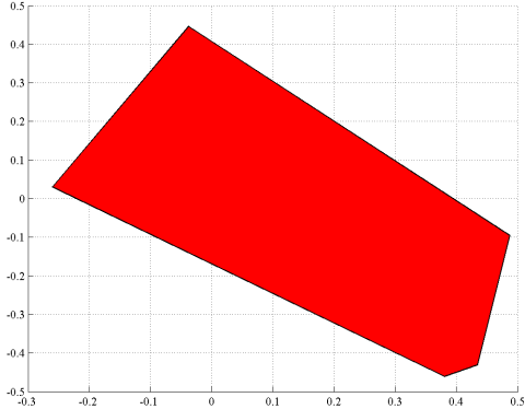
A cornerstone in MPT is the library for definition and manipulation of polytopes. Let us define a random polytope, and plot it using MPT.

A = randn(10,2);
b = 3*rand(10,1);
P = polytope(A,b);
plot(P);

The same plot can be achived by pure YALMIP code

x = sdpvar(2,1);
plot(A*x <= b);

Alternatively, we can use a combination of YALMIP and MPT. The result is the same YALMIP model as above.

plot(ismember(x,P));

A final approach is to define the problem using YALMIP code, but convert it to a polytopic object

plot(polytope(A*x <= b));

Note that the algorithm to plot the sets are completely different in YALMIP and MPT. MPT explicitly works with the polytopic structure and computes all vertices using a vertex enumeration algorithm. YALMIP on the other hand makes no assumption about the sets. To be able to handle arbitrary sets, it employs a ray-shooting strategy to generate points on the boundary of the feasible set, and then plot this (inner) approximation.

Minkowski difference

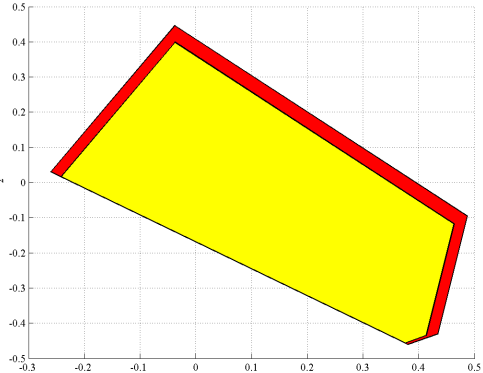
Minkowski difference, or polytope substraction, is overloaded on polytope objects in MPT. We define a new polytope, and subtract it from our first polytope

E = randn(10,2);
f = 0.1*rand(10,1);
S = polytope(E,f);
plot(P-S,'y');

To accomplish the same using only YALMIP, we have to go back to the defintion of the Minkowski difference. The Minkowski difference \(P-S\) is defined as all \(x\) such that \(x+w\) is in \(P\) for all \(w\) in \(S\). This can be interpreted as a robust optimization problem.

w = sdpvar(2,1);
plot([A*(x+w) <= b, E*w <= f, uncertain(w)]);

Once again, we implement this using a combination of YALMIP and MPT commands

plot([ismember(x+w,P), ismember(w,S), uncertain(w)]);

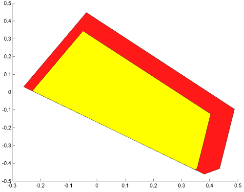
Note that the use of the [robust optimization framework] in YALMIP allows us to generalize the Minkowski difference to subtract an arbitrary conic set. MPT on the other hand is limited to polytopic sets.

w = sdpvar(2,1);
plot([A*(x+w) <= b, w'*w <= 0.08^2, uncertain(w)]);

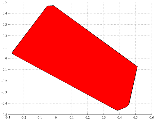
Minkowski sum

Addition of polytopes, i.e. Minkowski sum, is also directly available in MPT

plot(P+S)

Once again, to plot this using YALMIP, we use the definition of Minkowski sum, the set of all \(z\) such that \(z=x+w\) where \(x\) is in \(P\) and \(w\) is in \(S\). We thus create a new variable \(z\), use the definition, and plot the feasible set in the \(z\)-space.

z = sdpvar(2,1);
plot([z == x+w, A*x <= b, E*w <= f],z)

Chebychev balls

The Chebyshev ball is defined as the largest possible ball that can be placed inside a set \(P\). The search for the Chebychev center, and the associated size of the ball, can be stated as finding the largest \(r\) such that \(x+rd\) is in \(P\) for all \(d\) in a unit-ball.

In order to extend this concept, we first note that the Chebychev formulation can be interpreted as a robustness problem. Hence, we can compute the Chebychev ball using the robust optimization module

r = sdpvar(1);
xc = sdpvar(2,1);
d = sdpvar(2,1);
optimize([A*(xc+r*d) <= b, uncertain(d), d'*d <= 1],-r)

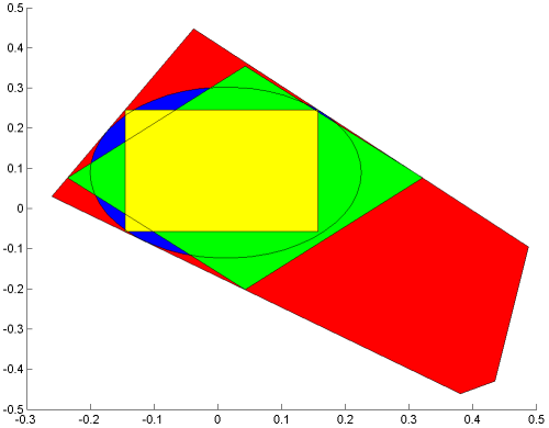
With this formulation at hand, we can generalize. The robust optimization module allows fairly general uncertainty descriptions when the uncertain constraint is elementwise. Let’s compute the 1-norm and infinity-norm Chebychev balls!

plot(A*x <= b);
optimize([A*(xc+r*d) <= b, d'*d <= 1, uncertain(d)],-r)
hold on
plot(norm(x-value(xc))<=value(r),x,'b')

optimize([A*(xc+r*d) <= b, norm(d,1)<=1, uncertain(d)],-r)
plot(norm(x-value(xc),1)<=value(r),x,'g')

solvesdp([A*(xc+r*d) <= b, norm(d,inf) <= 1, uncertain(d)],-r)
plot((abs(x-value(xc)))<=value(r),x,'y')

Projection

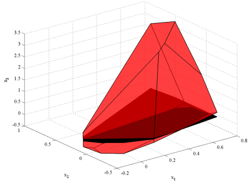
Define a polytope in 3D, and project it two its two first coordinates.

H = randn(10,3);
k = rand(10,1);
R = polytope(H,k);
plot(R);hold on
Q = projection(R,1:2);
plot(Q);

The same figure can be generated using YALMIP code

x = sdpvar(3,1);
plot(H*x <= k);hold on
plot(H*x <= k,x(1:2),'k');

Crucial to understand is that YALMIP does not explicitly generate any projection but simply plots the projection of the results from the ray-shooting.

However, if we want the explicit projection, the command projection is available on polytopic constraints. YALMIP will convert the constraints to an MPT polytope object, apply the projection, and the reconstruct a YALMIP constraint.

R = [H*x <= k]
Q = projection(R,x(1:2))
plot(R);hold on;
plot(Q,'k');

Slicing

MPT has support for slicing. This command allows you to fix the value of a set of variables, and plot the polytope in the remaining free variables. Let us fix the first coordinate to the value 0.2 in the 3D polytope above

plot(R);hold on;
plot(slice(R,1,0.2))

The same thing can be accomplished with the following YALMIP code. Note that we have to specify that we want to plot the remaning 2D polytope. Otherwise, YALMIP will try to plot a flat polytope in 3D

plot([H*x <= k, x(1)==0.2],x(2:3))

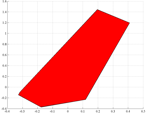
Alternatively, we can eliminate x(1) from the problem, and plot the 2D polytope that remains.

plot(replace(H*x,x(1),0.2) <= k)

Convex hull

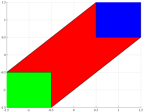
Both MPT and YALMIP can be used to obtain the convex hull of the union of polytopes. Using MPT, we quickly define two cubes and plot them and their convex hull

P1 = unitbox(2,0.5)+[1;1];
P2 = unitbox(2,0.5)+[-1;-1];
plot([hull([P1 P2]) P1 P2])

A pure YALMIP version would be

x = sdpvar(2,1);
P1 = -0.5 <= x-[1;1] <= 0.5;
P2 = -0.5 <= x+[1;1] <= 0.5;
P  = hull(P1,P2);
plot(P,x);hold on
plot(P1,x,'y');
plot(P2,x,'b');

Once again, note that MPT and YALMIP use different approaches to construct the convex hull. MPT is based on a vertex enumeration of the individual polytopes. YALMIP on the other hand is based on a general lifting approach involving additional variables and constraints (this is the reason we explicitly tell YALMIP to plot the convex hull w.r.t. the original variables, since auxiliary variables have been introduced). The benefit of this approach is of course that the method applies to arbitrary conic-representable sets as described in the convex hull command